KeywordsBenoit hypothesis defense spending Economic Growth external debt
JEL Classification B23, C32, O47
Full Article
1. Introduction
The issue of whether military expenditure interacts with the workings of economic forces to facilitate economic growth has received attention since pivotal submission of Benoit (1978). Theoretical postulations offer two opposing views by which defense spending and growth connect. The first, the Keynesian military view refers as the demand stimulation channel, argues that military expenditures are fragments of aggregate demand, therefore any increase in it increases employment, total output, and by implication result to rapid economic growth (Benoit, 1978). The second, the military spending detriment hypothesis, contends that growth leads to increased defense spending. The model assumes that defense spending generates opportunity cost and crowd out investment (Sandler and Hartley, 1995). Although the model recognized that military spending has known positive impacts (Waszkiewicz 2018), but the overall effect on growth is negative because of the trade-off of public resources.
Some authors have shown how military spending interacts with other variables to impact economic growth (Nikolaidou 2016; Waszkiewicz 2018; Dimitraki and Kartsaklas 2018; Ahmed, Mahmood and Shadmani, 2022; Kadim and Abbas, 2022; Topal, Unver, and Türedi, 2022; Zhang, Bouri, Klein, and Jalkh, 2022). Defense costs are associated with other economic problems, including global financial imbalance, inflation, and rising external debt (Waszkiewicz, 2018). Because many countries borrow to finance defense expenditure, it has been linked to increase external debts and debt crisis (Nikolaidou 2016). Such borrowing lowers consumption, therefore, may hinder growth potential (Dimitraki and Kartsaklas 2018). Ahmed et al. (2022) show that non-defense expenditure counter-cyclically reacts to output gap shocks, and shock to public debt may cause immediate rise in the non-defense spending, but later fall over the forecast horizon. Topal et al. (2022) explore panel heterogeneity and cross-sectional dependence of 27 NATO countries and find causality between military spending and growth. Zhang et al. (2022) examine co-movements between stock returns and risks in the aerospace and defense firms from ten countries and identify significant coherence joint movement around the outbreak of current Russia-Ukraine conflicts.
Available data show trend that Nigeria has increased its defense budget overtime. Various crisis such as border conflicts, ethnic clashes, insurgency, religious conflicts, kidnapping and terrorism, which the country continue to experience contributes to the rise in the defense spending. For the country, some studies examine the impact of military spending on growth (Temitope and Olayinka, 2021; Adekunle and Oyewole, 2022; Nwidobie, Audu, and Oni, 2022). Adekunle and Oyewole (2022) find that military spending negatively impacted growth in Nigeria between 1981 and 2020. Based on endogenous growth model, Nwidobie et al. (2022) identified significant positive (negative) relationship between growth and security expenditure in short-run (long-run). Temitope and Olayinka (2021) revealed significant positive long-run connection between growth and military expenditure for the country during 1981 – 2017.
The contending evidences has only focused on how defense spending affects growth, but fail to utilize the possibility of a unifying interactions between both, and amongst other variables, especially the increasing debts. The rationale behind the interconnectedness is that continuous spending to defend and curb domestic existential tensions are all more or less prone to mean shifts in public debts profile (Shabbir and Butt 2016; Abbas and Wizarat, 2018; Dudzevi, Cesnuityt, and Prakapien, 2021; Roth, Settele, and Wohlfart, 2021). These are believed to have far reached implications on economic growth (Ahmed, 2012; Casares, 2015; Pehlivan, Aysegül, Konat, 2021;). They are connected and are better analyzed jointly in a unifying framework. The joint analysis is important because economic growth and/or defense spending may not only affect public debts but may also react to public debt changes and vice versa. There is an urgent need to consider whether and how the heightened public debts, amid the rising defense spending, affects economic growth, and vice versa.
Motivated by the forgoing limitation and research gap, this paper aims to analyze the relations amongst defense spending, economic growth, and external debts under a joint and unifying framework. The paper considers a VAR model to examine the interconnectedness. For the aim, the VAR model is appropriate since it accommodates multi-policy shock, multi-variables (such as the defense spending, public debts and economic growth) as well as multi-equations or policy reaction functions, all within one framework. The unified framework controls for exogenous policy actions and reactions of the considered variables. The policy actions on one may generate observed co-movements of the other.
The results show evidence of a lot of interactions among the variables, which supports the unified analysis applied for the paper. The significance of considered model’s crucial coefficients demonstrates that the increase in economic growth would be accompanied by increase in defense spending. The findings show economic growth leads to a significant increase (decrease) in the current value of defense spending (debt), and more so, increased debt creates pressure that may ignite next period growth. Besides enriching the literature regarding the interconnectedness of economic growth, defense spending and public debt, the paper offers new insights useful for understanding how shocks in defense spending heightened external debt profiles and economic growth prospects.
2. Methodology
2.1. Data
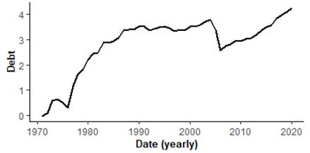
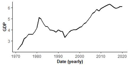
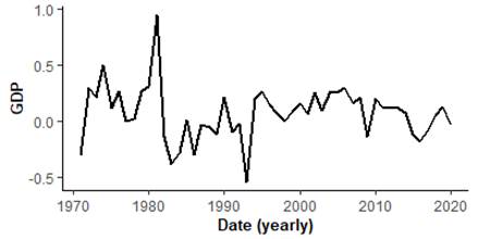
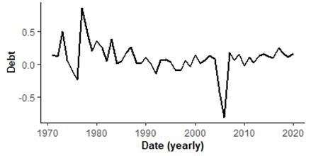
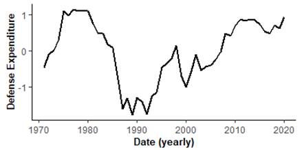
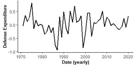
The study obtained data on the Nigeria GDP, military expenditure and external debts for period covering 1971–2020, from the World Bank database. The series are log normalized (i.e., natural log-transformed) before been used for estimation to minimize heteroscedasticity, and more so, to ensure the estimators are insensitive to the data and unequal estimates (Mills, 2019). The log-scaled usually mildly smoothen possible spikes and tractions relative to the actual observations (Gbadebo et al., 2021). Figures 1 and 2 depict the time series plot (levels and difference) for series. Visibly, GDP and external debts are clearly drifted, upward trended, likely negative skewed and indicating sign for nonstationary. The log difference variables are closely mean reversing. Since 1990, the defense expenditure appears more trended, but overall, the unit root tests are applied confirmed for the log-transformed series.
| Figure 1. Log-scale | Figure 2. Log-difference | ||
| Panel a: GDP | |||
|
|
||
| Panel b: Debt | |||
|
|
||
| Panel c: Defense expenditure | |||
|
|
||
Figures 1-2. Time series plots in level (differenced) forms
2.2. Method
2.2.1 The Stationarity and Cointegration Tests
The stationarity and unit root test confirms the stochastic characterization of data generating process of the gross domestic product (![]() ), defense spending (
), defense spending (![]() ) and external debts (
) and external debts (![]() ) based on the Augmented-Dickey-Fuller (ADF) test. Let
) based on the Augmented-Dickey-Fuller (ADF) test. Let ![]() represents each series, the generic ADF uses equation (1) to verify stationarity for
represents each series, the generic ADF uses equation (1) to verify stationarity for ![]() :
:
![]()
With: ![]() The drift, white noise and lag length are respectively,
The drift, white noise and lag length are respectively, ![]() and
and ![]() . The measure
. The measure ![]() is the ADF statistic (where
is the ADF statistic (where ![]() =
=![]() ’s standard error), and it is compared with the ADF critical value (
’s standard error), and it is compared with the ADF critical value (![]() ). The test is performed with the null of non-stationarity (
). The test is performed with the null of non-stationarity (![]() ) and alternative (
) and alternative (![]() . The test identifies the series as I(0), for stationarity at level or as
. The test identifies the series as I(0), for stationarity at level or as ![]() , order of integration), for
, order of integration), for ![]() -differenced stationarity. The procedure must complete the optimal lag per variable under consideration to obtain white noises in each (Bueno, 2015). Afterward, the study selects the system’s optimal lag (
-differenced stationarity. The procedure must complete the optimal lag per variable under consideration to obtain white noises in each (Bueno, 2015). Afterward, the study selects the system’s optimal lag (![]() ) for the parsimonious parameterisation of the cointegration. If
) for the parsimonious parameterisation of the cointegration. If ![]() ’s are confirmed integrated [e.g.,
’s are confirmed integrated [e.g., ![]() ], the study applies the Johansen cointegration (Hamilton, 2020).
], the study applies the Johansen cointegration (Hamilton, 2020).
The Johansen test applies the Maximum Likelihood Estimation for a cointegrated system. If at least vector ![]() in the system of dimension n is
in the system of dimension n is ![]() , and
, and![]() is
is ![]() then any arbitrary linear combination of the elements of
then any arbitrary linear combination of the elements of ![]() such as
such as ![]() , where matrix
, where matrix ![]() will be
will be![]() . If there exist vectors
. If there exist vectors ![]() , such that
, such that ![]() then the components of
then the components of ![]() are co-integrated. For any nonsingular
are co-integrated. For any nonsingular ![]() matrix
matrix ![]()
![]() is I(0), r(rank) is the number of co-integrating relationships. Consider the (linear) system equation with no deterministic terms:
is I(0), r(rank) is the number of co-integrating relationships. Consider the (linear) system equation with no deterministic terms:
![]()
![]() , ... ,
, ... , ![]() (2)
(2)
The Johansen cointegration test verify rank (r) of the cointegrating space of matrix ![]() [
[![]() and
and ![]() are
are ![]() , where Vector
, where Vector ![]() contains both
contains both ![]() and
and ![]() Both Trace and Maximum eigenvalue are used to determine the rank. The Trace [Maximum eigenvalue] null of no co-integrating vectors [
Both Trace and Maximum eigenvalue are used to determine the rank. The Trace [Maximum eigenvalue] null of no co-integrating vectors [![]()
![]() ] is tested against the alternative hypothesis of at least one co-integrating vector [
] is tested against the alternative hypothesis of at least one co-integrating vector [![]() : r > 0]. The Trace statistic (
: r > 0]. The Trace statistic (![]() : equation 10) and Maximum eigenvalue (
: equation 10) and Maximum eigenvalue (![]() : equation 11, where
: equation 11, where ![]() are the
are the ![]() smallest squared canonical correlations between
smallest squared canonical correlations between ![]() (
(![]() ) and
) and ![]() , are defined.
, are defined.
2.2.2. VAR/VECM, IRF and FEVD
This paper aims to analyze the relations amongst defense spending, economic growth, and public debts under a joint and unifying framework. The paper considers the vector autoregression (VAR/VECM) to examine the interconnectedness. The vector autoregression approach accommodates multi-policy shock, multi-variables and multi-equations or policy reaction functions to depict the dynamic links of considered variables within same framework. The models show how endogenous variables are explained by own pasts, as well as the pasts and current value of the regressors.
The ![]() , for instance, holds set of
, for instance, holds set of ![]() endogenous variables
endogenous variables ![]() . The
. The ![]() -process is:
-process is:
![]() (5)
(5)
Where, ![]() (
(![]()
![]() ,
, ![]() ) represent
) represent ![]() coefficient matrices,
coefficient matrices, ![]() is a
is a ![]() -dimensional process with
-dimensional process with ![]() and covariance matrix
and covariance matrix ![]() (white noise). The VAR(p)-process has empirical features of ‘stability’, which is analyzed by computing the eigenvalues of
(white noise). The VAR(p)-process has empirical features of ‘stability’, which is analyzed by computing the eigenvalues of ![]() in the VAR(p)-process compact moving average (MA) form.
in the VAR(p)-process compact moving average (MA) form.
![]() , (6)
, (6)
![]()
![]() ,
, 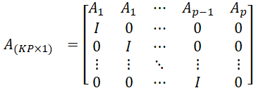 ,
, 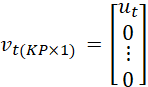 (7)
(7)
A is a matrix of dimension ![]() , while
, while ![]() and
and ![]() are stacked vectors of dimension
are stacked vectors of dimension ![]() . The
. The ![]() system is stable, if the absolute figures of the eigenvalues of
system is stable, if the absolute figures of the eigenvalues of ![]()
![]()
In the computation, if established that the variables in the VAR are cointegrated, the empirical process procedure becomes appropriate to depict the VECM. Unlike the VAR, the VECM includes an error correction term that identifies reactions to equilibrium’s deviation due to perturbations. Based on (Pfaff, 2006), the VAR model (5) is transformed to specify the VECM, which specification can either be made to signify the cumulative ‘long-run’ impacts (equation 8) or alternatively the ‘transitory’ effects (equation 9).
![]()
With; ![]() ,
, ![]()
![]() ,
,
![]()
![]()
![]()
![]() .
.
![]()
Equation (8) signifies the long-run form and ![]() encloses the ‘long-run’ impacts, whereas (9) (9) is signified as ‘transitory’ form, for which
encloses the ‘long-run’ impacts, whereas (9) (9) is signified as ‘transitory’ form, for which ![]() measures transitory effects. For cointegration case,
measures transitory effects. For cointegration case, ![]() is of reduced rank (
is of reduced rank (![]() ). The dimensions of
). The dimensions of ![]() and
and ![]() is
is ![]() .
. ![]() is loading matrix, while estimates of the long-run equilibrium are loaded in
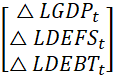
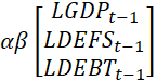
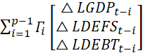
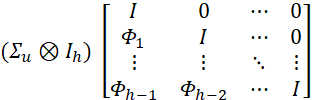
is loading matrix, while estimates of the long-run equilibrium are loaded in ![]() . Applying the equation 8 for the study’s specific data and relationship amongst the gross domestic product, defense spending, external debts, and including the constant (c), the paper estimate:
. Applying the equation 8 for the study’s specific data and relationship amongst the gross domestic product, defense spending, external debts, and including the constant (c), the paper estimate:
![]()
![]() +
+ 
![]()
![]() (11)
(11)
For the aim, the paper present a three-equation model with three variables that extracts the policy shocks and policy reaction functions all within one framework. The IRF and FEVD diagnose the models’ dynamic behavior. Both aligns with the Wold MA representation (6) for stable ![]() -process:
-process:
![]() (12)
(12)
with ![]() and
and ![]() computed recursively using,
computed recursively using, ![]()
![]() (for
(for ![]()
![]() ,), whereby
,), whereby ![]() for
for ![]() The forecasts for horizons
The forecasts for horizons ![]() of the
of the ![]() -process is recursively generated from:
-process is recursively generated from:
![]()
![]() , (11)
, (11)
Where, ![]() for
for ![]() . The forecast error covariance matrix is:
. The forecast error covariance matrix is:
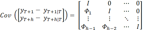
![]() is the Kronecker operator, and matrices
is the Kronecker operator, and matrices ![]() are the coefficient matrices of the Wold MA decomposition of a stable
are the coefficient matrices of the Wold MA decomposition of a stable ![]() -process. The estimation was completed based on procedure in Pfaff and Taunus (2020), and implemented within the R Package ‘vars’, which utilizes basic R-commands.
-process. The estimation was completed based on procedure in Pfaff and Taunus (2020), and implemented within the R Package ‘vars’, which utilizes basic R-commands.
3. Results
Before the main analysis, preliminary evaluations are completed to report the summary statistics and the correlation coefficients, as well as to confirm the stochastic feature of DGP of the considered variables. Table 1 (Table 2) reports the basic statistics (unit root test) for the natural log of gross domestic product (![]() ), defense spending (
), defense spending (![]() ) and external debts (
) and external debts (![]() ). The data establish positive between GDP and defense spending (0.42) as well as between GDP and debt (0.58). Negative correlation (-0.31) is found between defense spending and external debts. All the correlation coefficients are found significant, suggesting sturdy GDP-defense spending co-movement tendency. The causal relationships suppose that economic growth relates to information about the trended defense spending in Nigeria, and vice versa. Hence, specific growth shocks may be accountable for a certain increase in the defense spending episodes. The result, from ADF implemented (Table 2), reveals that all three variables are non-stationary, in I(0), but are different stationary [I(1)], supposing they integrated. With
). The data establish positive between GDP and defense spending (0.42) as well as between GDP and debt (0.58). Negative correlation (-0.31) is found between defense spending and external debts. All the correlation coefficients are found significant, suggesting sturdy GDP-defense spending co-movement tendency. The causal relationships suppose that economic growth relates to information about the trended defense spending in Nigeria, and vice versa. Hence, specific growth shocks may be accountable for a certain increase in the defense spending episodes. The result, from ADF implemented (Table 2), reveals that all three variables are non-stationary, in I(0), but are different stationary [I(1)], supposing they integrated. With![]()
![]() at level for the different series, the test (with or without trends in the test equation) fail to reject the null of non-stationarity for all variables. Not surprising, the time series plots clearly identify that although both GDP and debts are trended, while the defense spending overall likely drifted but trended since 1990, the representative log-difference (Figure 2a, 2b, 2c) are visibly mean reversing.
at level for the different series, the test (with or without trends in the test equation) fail to reject the null of non-stationarity for all variables. Not surprising, the time series plots clearly identify that although both GDP and debts are trended, while the defense spending overall likely drifted but trended since 1990, the representative log-difference (Figure 2a, 2b, 2c) are visibly mean reversing.
To avoid over-parameterization and ensure the system’s parametric parsimony, we confirm the optimal lag, and report the results in Table 3. The outcome indicates that the three major lag selection criteria (HQ, AIC and SC) unanimously suppose an optimal lag of 1 is likely more parsimonious for the parameterization of the cointegration. The paper completes the robustness check [Table 4] to decide the efficient system for construction of the impulse response. The stability tests for the time-invariant estimation shows that there is no deviations from the anticipated parameter constancy, therefore the model holds for the cointegration test. Both Trace and Max-Eigen tests are applied and the outcome reported in Table 4. Each test is not signficant (![]() -value=95%) at the cointegration rank of 2. The result supposes only 2 co-integrating combinations at 5%. The Trace test statistics (
-value=95%) at the cointegration rank of 2. The result supposes only 2 co-integrating combinations at 5%. The Trace test statistics (![]() ) and maximum-eigenvalue statistics (
) and maximum-eigenvalue statistics (![]() ) are much lower than the respective critical value, both been 3.842 at r = 2. Since cointegrating ranks do exist amongst the GDP, defense spending and debts, the VECM becomes more suitable to depict the system interdependence based on the unifying framework for making statistical inference for the relationship.
) are much lower than the respective critical value, both been 3.842 at r = 2. Since cointegrating ranks do exist amongst the GDP, defense spending and debts, the VECM becomes more suitable to depict the system interdependence based on the unifying framework for making statistical inference for the relationship.
Table 1: Basic Statistics and unit root test
| Variable | Summary Statistics | Correlation Coefficients a | ||||||
|
|
|
|
|
|
|
|
|
|
|
|
4.55 | 1.10 | 2.03 | 0.36 | 1 | |||
|
|
0.01 | 0.85 | 3.49 | 0.17 | 0.42** | 1 | ||
|
|
2.83 | 1.10 | 17.23 | 0.00 | 0.58* | -0.31** | 1 | |
Note: ![]() ean (
ean (![]() ), Standard deviation (
), Standard deviation (![]() ), Jarque-Bera statistics (JB) p-value of JB statistics (Prob).
), Jarque-Bera statistics (JB) p-value of JB statistics (Prob).
b Only the first difference of each series of ![]() is reported.
is reported.
*,**,*** shows statistical significance using probability p![]() , at 1%, 5% or 10% significance levels, respectively. The data establish positive between GDP and defense spending (0.42) as well as between GDP and debt (0.58). Negative correlation (-0.31) is found between defense spending and external debts. All the correlation coefficients are found significant.
, at 1%, 5% or 10% significance levels, respectively. The data establish positive between GDP and defense spending (0.42) as well as between GDP and debt (0.58). Negative correlation (-0.31) is found between defense spending and external debts. All the correlation coefficients are found significant.
Table 2: Stationarity test for the data
|
Variable [ |
Lag | Test |
Critical values [ |
||
| Deterministic terms | Length |
value |
0.01 | 0.05 | 0.1 |
| LGDP | |||||
| Intercept | 2 | -1.68 | -3.57 | -2.92 | -2.60 |
| Intercept and Trend | 3 | -2.08 | -4.16 | -3.51 | -3.18 |
| Trend | 1 | -5.23 | -3.57 | -2.92 | -2.60 |
| LDEFS | |||||
| Intercept | 2 | -1.32 | -3.57 | -2.92 | -2.60 |
| Intercept and Trend | 2 | -1.34 | -4.16 | -3.50 | -3.18 |
| Trend | 1 | -6.37 | -3.57 | -2.92 | -2.60 |
| LDEBT | |||||
| Intercept | 2 | -2.69 | -3.57 | -2.92 | -2.99 |
| Intercept and Trend | 3 | -2.16 | -4.16 | -3.50 | -3.18 |
| Trend | 1 | -5.22 | -3.57 | -2.92 | -2.60 |
Note: The Bold figures re the first difference tests. The ADF statistic (![]() ) is compared with the ADF critical value (
) is compared with the ADF critical value (![]() ]) from MacKinnon (1996) one-sided p-values, at the different level significance. The test is completed with the null of non-stationarity (
]) from MacKinnon (1996) one-sided p-values, at the different level significance. The test is completed with the null of non-stationarity (![]() ) and alternative (
) and alternative (![]() . With
. With![]()
![]() at level for the different series, the result in Table 3 reveals that the 3 variables are differenced stationary and integrated [I(1)].
at level for the different series, the result in Table 3 reveals that the 3 variables are differenced stationary and integrated [I(1)].
Table 3: Optimal lag selection for the cointegration parameterization
| Selection | Lag Length | ||||
| Criteria | 1 | 2 | 3 | 4 | 5 |
| AIC(n) | -8.21* | -8.11 | -7.78 | -7.78 | -7.94 |
| HQ(n) | -7.98* | -7.75 | -7.28 | -7.15 | -7.18 |
| SC(n) | -7.60 | -7.15 | -6.45 | -6.10 | -5.89 |
| FPE(n) | 0.00 | 0.00 | 0.00 | 0.00 | 0.00 |
Note: Final Prediction Error (FPE), Akaike Information Criterion (AIC), Schwarz Criterion (SC) and Hannan Quinn (HQ) Criterion. The diagnostic tests are performed to decide the most parsimonious lag for the dynamics of the system’s estimation. * Selected optimal lag ![]() based on the corresponding selection criteria.
based on the corresponding selection criteria. ![]() is the number of lag implemented during the specific criterion iteration. All three major lag selection criteria (HQ, AIC and SC) unanimously suppose lag 1 as optimal.
is the number of lag implemented during the specific criterion iteration. All three major lag selection criteria (HQ, AIC and SC) unanimously suppose lag 1 as optimal.
Table 4: Cointegration test for the relations
|
Hypothesized No. of CE(s) |
Critical Value (0.05) |
|||
| Eigenvalue | Statistic |
|
||
|
Trace
[ |
||||
| None * | 0.84 | 105.024 | 29.806 | 0.000 |
| At most 1 * | 0.57 | 33.185 | 15.496 | 0.000 |
| At most 2 | 0.00 | 0.001 | 3.842 | 0.951 |
|
Max-Eigen
[ |
||||
| Max-Eigen | ||||
| None * | 0.84 | 71.842 | 21.135 | 0.000 |
| At most 1 * | 0.57 | 33.185 | 14.286 | 0.000 |
| At most 2 | 0.00 | 0.001 | 3.842 | 0.951 |
Note: * denotes rejection of the hypothesis at the 0.05 level. Selected (0.05 level*) number of Cointegrating Relations. The Johenson test completed, using optimal lag of 1, implements linear trend for data. Both Trace and Max-eigenvalue test statistics indicate 2 cointegrating equations at the 0.05 level for most tests.
The VEC model, estimated at the optimal lag of the cointegrating regression relates the endogenous variables (economic growth, defense spending and public debts) in the three different models, while estimating the long-run estimates amongst them and the vector error correction. The interdependence dynamics is computed with a deterministic trend included in the cointegration relation. Based on the Wald test completed, the estimation is parsimonious as no variable is found redundant. The empirical computation identifies equation (11) as:
![]() +
+  +
+ 
![]()
![]() (11)
(11)
Table 5 presents the cointegration matrix’ coefficients ![]() of the error correction (EC) component, and Table 6 reports the adjustment coefficients (
of the error correction (EC) component, and Table 6 reports the adjustment coefficients (![]() ,
, ![]() ) of the EC term. The adjustment coefficient
) of the EC term. The adjustment coefficient ![]() , which is negative in the equation
, which is negative in the equation ![]() , applies to the cointegration matrix
, applies to the cointegration matrix ![]() . Analyzing the model, the coefficient of
. Analyzing the model, the coefficient of ![]() is positive in
is positive in ![]() , indicating that a rise of
, indicating that a rise of ![]() in t-1, not followed by proportional increase in the public debt that more than likely neutralizes the increase, signifies a deceleration in the current value of
in t-1, not followed by proportional increase in the public debt that more than likely neutralizes the increase, signifies a deceleration in the current value of ![]() since
since ![]() [ = -0.06, in Table 6] is negative. Conversely, the coefficient of
[ = -0.06, in Table 6] is negative. Conversely, the coefficient of ![]() is negative in
is negative in ![]() , supposing that an increase
, supposing that an increase ![]() , without simultaneous increase in current value of
, without simultaneous increase in current value of ![]() , and/or change in the defense spending, creates pressure such that in the next period the variation of
, and/or change in the defense spending, creates pressure such that in the next period the variation of ![]() would increase.
would increase.
Similarly, the adjustment coefficient ![]() , which is also negative in the
, which is also negative in the ![]() equation, applies to the cointegration matrix
equation, applies to the cointegration matrix ![]() . The analyzing infer that defense spending coefficient is positive in
. The analyzing infer that defense spending coefficient is positive in ![]() , and by implication a rise of
, and by implication a rise of ![]() in t-1, not accompanied by increase in the debt (
in t-1, not accompanied by increase in the debt (![]() ) that may neutralizes the increase, signifies a decline in the current value of spending on defense since
) that may neutralizes the increase, signifies a decline in the current value of spending on defense since ![]() [= -0.09] is negative. The coefficient of debts is negative in
[= -0.09] is negative. The coefficient of debts is negative in ![]() , supposing that an increase
, supposing that an increase ![]() , without proportional increase in defense spending, creates pressure such that in the next period the variation of
, without proportional increase in defense spending, creates pressure such that in the next period the variation of ![]() would increase.
would increase.
The adjustment coefficient of the error correction, ![]() , is negative in the growth equation and highly significance at 1%, supposing that deviation from the long-term dynamics triggered by shock of the variables is minimized by 6% (been the correction based on
, is negative in the growth equation and highly significance at 1%, supposing that deviation from the long-term dynamics triggered by shock of the variables is minimized by 6% (been the correction based on ![]() ) in the next year. The adjustment coefficient
) in the next year. The adjustment coefficient ![]() and
and ![]() contribute to around 40% and 60%, respectively, for long-term dynamics in the LGDP equation.
contribute to around 40% and 60%, respectively, for long-term dynamics in the LGDP equation. ![]() , is also negative and highly significance in the defense spending and debt equations, inferring deviation from the long-term dynamics are minimized, with
, is also negative and highly significance in the defense spending and debt equations, inferring deviation from the long-term dynamics are minimized, with ![]() and
and ![]() contributing 42.6% and 57.4% for long-term dynamics in the debt equation, and 14.3% and 85.7% for long-term dynamics in the defense spending equation. The surge in defense spending beyond the equilibrium constraints in preceding period are adjustable by the modifier error correction to revert and maintain the system’s equilibrium. As noted (Engle and Granger, 1987), known deviations from the equilibrium of the autoregression system due to perturbations of system’s variables are minimized with the correction.
contributing 42.6% and 57.4% for long-term dynamics in the debt equation, and 14.3% and 85.7% for long-term dynamics in the defense spending equation. The surge in defense spending beyond the equilibrium constraints in preceding period are adjustable by the modifier error correction to revert and maintain the system’s equilibrium. As noted (Engle and Granger, 1987), known deviations from the equilibrium of the autoregression system due to perturbations of system’s variables are minimized with the correction.
Table 5: Cointegration Matrix (β)’s Coefficients
|
|
|
|||||
| Variable | ||||||
|
|
1 | - | - | - | - | - |
|
|
- | - | - | 1 | - | - |
|
|
-3.58 | 0.92 | -3.91* | -1.92 | 0.62 | -3.08* |
Note: *indicates statistical significance at 1%.
Table 6: VECM regressions’ Coefficient
|
Error Correction: |
|
|
|
||||||
|
|
|
|
|
|
|
|
|
|
|
| C | 0.05* | 0.04 | 0.001 | -0.01** | 0.06 | 0.034 | 0.10* | 0.04 | 0.007 |
|
|
0.22 | 0.15 | 0.150 | 0.26*** | 0.23 | 0.072 | -0.18* | 0.14 | 0.008 |
|
|
0.08** | 0.10 | 0.025 | 0.13*** | 0.15 | 0.099 | -0.16*** | 0.09 | 0.074 |
|
|
0.05*** | 0.16 | 0.080 | 0.12 | 0.25 | 0.123 | 0.08 | 0.15 | 0.610 |
|
|
-0.06* | 0.06 | 0.004 | -0.23* | 0.08 | 0.008 | -0.01*** | 0.05 | 0.071 |
|
|
-0.09** | 0.08 | 0.018 | -0.31* | 0.11 | 0.008 | 0.06** | 0.07 | 0.032 |
| Statistics | |||||||||
|
|
0.85 | 0.69 | 0.63 | ||||||
|
|
1.51 | 2.03 | 3.53 | ||||||
Note: *p<0.1; **p<0.05; ***p<0.01.
Analyzing the variables of the VECM, Table 6 indicate they are significance except for ![]() , in the economic growth equation and
, in the economic growth equation and ![]() in both defense spending and debt equations. The significance indicate the stability of the long-run estimates, and also the short-run dynamics are sustained to the convergence long-run cointegrating equation. The system identifies that the cointegration relation has a reverse shock effects. The analysis shows that the coefficients of defense spending and external debt are in the
in both defense spending and debt equations. The significance indicate the stability of the long-run estimates, and also the short-run dynamics are sustained to the convergence long-run cointegrating equation. The system identifies that the cointegration relation has a reverse shock effects. The analysis shows that the coefficients of defense spending and external debt are in the ![]() regression are positive, equal to 0.08 and 0.05, and significant only at 5% and 10%, respectively. In this sense, a 1% increase in defense spending (debt) lead to a yearly increase of 8% (5%) in growth, in the following year.
regression are positive, equal to 0.08 and 0.05, and significant only at 5% and 10%, respectively. In this sense, a 1% increase in defense spending (debt) lead to a yearly increase of 8% (5%) in growth, in the following year.
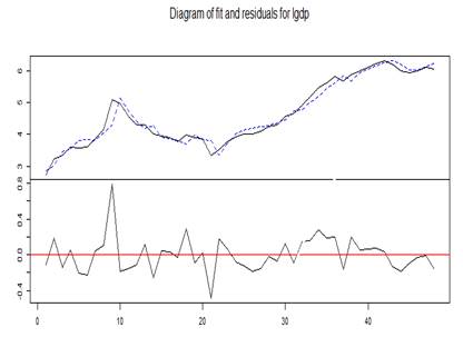
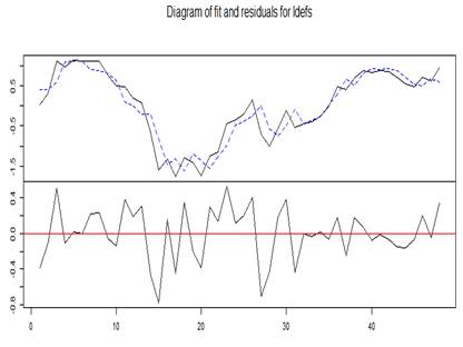
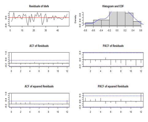
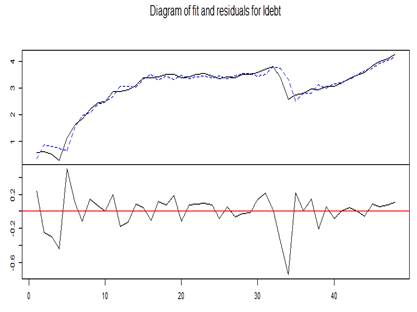
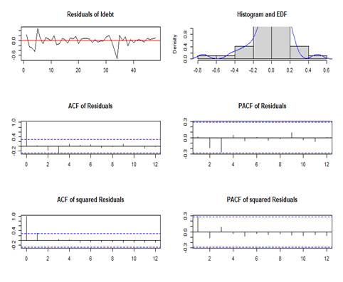
Table 7 show the outcomes of the diagnostic tests for the parsimonious model is provided, and Figure 3 (Panel a – c) depict the plots of residuals and the multivariable ARCH for the gross domestic product (![]() ), defense spending (
), defense spending (![]() ) and external debts (
) and external debts (![]() ). The diagnostic confirms the adequacy of the model. The model residuals’ histograms depict a near zero concentration of observations with progressive frequency decline along the tails of the equations of the VECM system. The possible existence of serial correlation of multivariate residuals is checked based on the Portmanteau (2006) test, and the null of no serial correlation is not refuted. Except for one, all Eigen values are encircled within a unit circle, hence further inferring system stability. This s further supported by the OLS-CUSUM visualisation tests for the different equations in the VECM (Figure 4). The estimates fall inside the critical bands indicating the stability of the long run coefficients.
). The diagnostic confirms the adequacy of the model. The model residuals’ histograms depict a near zero concentration of observations with progressive frequency decline along the tails of the equations of the VECM system. The possible existence of serial correlation of multivariate residuals is checked based on the Portmanteau (2006) test, and the null of no serial correlation is not refuted. Except for one, all Eigen values are encircled within a unit circle, hence further inferring system stability. This s further supported by the OLS-CUSUM visualisation tests for the different equations in the VECM (Figure 4). The estimates fall inside the critical bands indicating the stability of the long run coefficients.
Table 7: Diagnostic tests are conducted for the model.
| Serial Correlation | ARCH | Normality | |
| (Portmanteau test) | (M-Arch) | (JB-Test) | |
|
|
123.09 | 174.34 | 65.217 |
|
|
(0.000566) | (0.001605) |
(3.90 |
Note: Value in parenthesis are p-value. The VEC serial correlation fail to reject the null of absence of serial correlation. The MARCH test is significant, so residuals is not heteroscedastic. The Jarque-Bera statistic fail reject the multivariate normality for the stochastic errors. * indicates statistical significance at 1%.
|
Panel a: Residuals and multivariable ARCH’s plots for gross domestic product ( |
|
|
|
|
Panel b: Residuals and multivariable ARCH’s plots for defense spending ( |
|
|
|
|
Panel c: Residuals and multivariable ARCH’s plots external debts ( |
|
|
|
Figure 3: The plots of residuals and multivariable ARCH for gross domestic product (![]() ), defense spending (
), defense spending (![]() ) and external debts (
) and external debts (![]() )
)
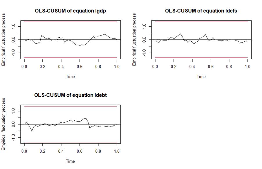
Figure 4: OLS-CUSUM Plots
Note: Estimates fall inside the critical bands (red lines), hence the long-run coefficients are stable. Source: Author (2023)
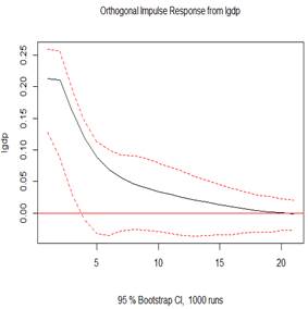
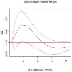
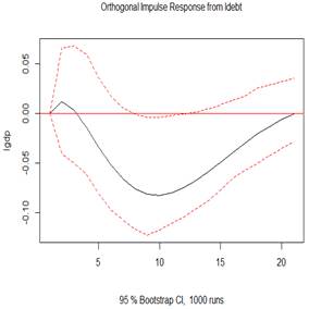
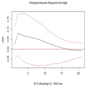
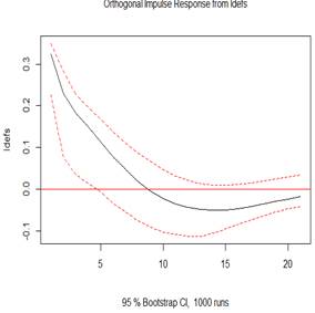
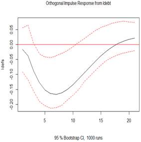
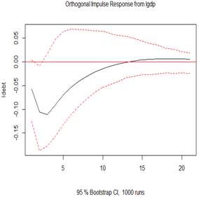
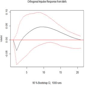
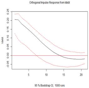
Figure 4 (top 3 plots) depicts the orthogonal impulse response of GDP to shocks in GDP, defense spending shock and external debt. The evidence observes economic growth rises on impact, but keeps falling gradually until the 20th year, which is statistically significant. The 100% shocks on GDP generates an initial increase impulse response at about 22% in GDP, in the subsequent year. The shock indicates a positive response for economic growth even up to the 20 years. The perturbation in the growth would later decline speedily within the first five years, and gradually in the following 15 years. The 100% shocks on defense spending does not generates any initial increase impulse response in GDP but presents a gradually and positive increase for GDP within the first five years, and gradual fall but still increase up till the twelfth year, when it no longer become statistically significant. The 100% shocks on presents a rise in GDP on impact and is significant within two years. From the 3rd year, there was a drop, which extended till the 10th year, after which a reverse and rise was observed again and onward but is not statistically significant. This finding implies economic growth depicts counter cyclicality albeit briefly due to defense spending shock, but extended due to debt shock.
|
|
|
|
|
|
|
|
|
Figure 5: Plots of the impulse response function (IRF)
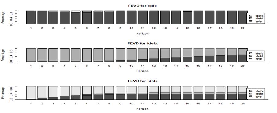
Figure 6: Forecast error variance decomposition (FEVD)
Source: World Bank Data | Author's R-‘vars’ Package outputs (2023)
4. Conclusions
How military expenditure interacts with other economic forces to bring about economic growth has gain attention of researcher. Because of increasing trend in military expenditure and defense spending a very limited studies for Nigeria have investigate the relationship and found mixed results (Temitope and Olayinka, 2021; Nwidobie et al, 2022). While existing evidence might agree positive or negative influence of defense spending on growth and thereby, assist to frame closely realistic situation in the inclusion of growth debt (Abbas and Wizarat, 2018; Roth et al., 2021). Hence, a joint and unifying framework is linked for defense spending, economic growth, and debt in Nigeria to control for exogenous policy actions and reactions amongst them. The cointegration test makes it possible to confirm the tendency of simultaneous rise or decline amongst economic growth, defense spending and external debts. Because the considered variables are confirmed non-stationary, and the relations cointegrated, the study presents the interconnectedness with the VECM approach to observe a strong unified relationship for the variables.
The findings identify long-term dynamics for the relationship, and that economic growth leads to a significance increase (decrease) in the current value of defense spending (debt), Moreso, increase debt creates pressure that may ignite next period growth. Besides enriching the literature regarding the interconnectedness of economic growth, defense spending and public debt, the paper offers new insights useful for understanding how shocks in defense spending heightened external debt profiles and economic growth prospects. This is the case for the Keynesian military view of growth nexus, which considers that military spending leads to output growth. Because military expenditures are fragments of aggregate demand, any increase in it increases employment, total output, and by implication results to rapid economic growth.
The study only considers how defense spending affect growth from a country’s aggregate perspectives, and was not investigated for firm-by-firm effect. This issue needs different in-depth investigation and might be a subject of research in the future. Research can build on the findings to optimize investment in military hardware generates employment in the defense sector, and how country growth increases firm level defense portfolios. Another extension for the paper is to cover broader areas including to involve other countries for a panel work. The interpretation of the outcomes for such would permit making more inferences regarding the spatial effect of geopolitical risk on defense spending and growth.
---
Author Contribution: The author solely completes all sections, including the Conceptualization, Investigation, Methodology, Visualization, Data Curation, Formal Analysis and the Drafting.
Acknowledgements: I thank Professor O. J. Akande and Dr A. O. Adekunle for their mentorship as well as Walter Sisulu University, for various levels of support leading to the completion of this work, and others.
Funding: This research received no external funding.
Conflicts of Interest: The author states that there are no conflicts of interest.
References
- Abbas, S. and Wizarat, S., 2018. Military expenditure and external debt in South Asia: A panel data analysis. Peace Economics, Peace Science and Public Policy, 24 (3), pp.1–7. https://doi.org/10.1515/peps-2017-0045.
- Casares, E.R., 2015. A relationship between external public debt and economic growth. Estudios Económicos, 30 (2), pp. 219–243. https://ideas.repec.org/a/emx/esteco/v30y2015i2p219-243.html.
- Adekunle, J.K. and Oyewole, O., 2022. Nexus between military expenditure, national insecurity and economic growth in Nigeria, International Journal of Economics, Commerce and Management, X (9), pp.290–298. https://ijecm.co.uk/wp-content/uploads/2022/09/10919.pdf.
- Ahmed, A.D., 2012. Military spending and growth in sub-Saharan Africa: A dynamic panel data analysis. Defense and Peace Economic, 23 (5), pp.485–506. https://doi.org/10.1080/10242694.2011.627163.
- Ahmed, H.A., Mahmood, S. and Shadmani, H., 2022. Defense and non-defense vs debt: How does defense and non-defense government spending impact the dynamics of federal government debt in the United States? Journal of Government and Economics, 7 (Autumn), pp.100050. https://doi.org/10.1016/j.jge.2022.100050.
- Ahmed, S. and Kamran, A., 2017. Impact of military spending on external debt in indebt developing countries: A cross country analysis. Tenth International Conference on Management Science and Engineering Management, 24 August 2016, Advances in Intelligent Systems and Computing, Singapore: Springer, pp.1505–1515. https://doi.org/10.1007/978-981-10-1837-4_122.
- Benoit, E., 1978. Growth and defense in developing countries. Economic Development and Cultural Change, 26 (2), pp.271–280. http://www.jstor.org/stable/1153245.
- Bueno, R., 2015. Econometria de séries temporais. 3rd ed. Sao Paulo, Brazil: Cengage Learning, pp.201–23.
- Dimitraki, O. and Kartsaklas, A., 2018. Sovereign debt, deficits and defense spending: The case of Greece. Defence and Peace Economics, 29 (6): 712–727. http://dx.doi.org/10.1080/10242694.2017.1289497.
- Dudzevic, G., Cesnuityt, V. and Prakapien, D., 2021. Defence expenditure-government debt nexus in the context of sustainability in selected small European union countries. Sustainability, 13 (12), pp.1–18. https://doi.org/10.3390/su13126669.
- Gbadebo, A.D., Adekunle, A.O., Adedokun, M., Lukeman, A.A. and Akande, J., 2021. BTC price volatility: Fundamentals versus information. Cogent Business and Management, 8(1), pp.1984624. https://doi.org/10.1080/23311975.2021.1984624.
- Hamilton, J., 2020. Time Series Analysis. 2nd ed. New Jersey, United States: Princeton University Press, pp.571–629.
- Kadim, N.J. and Abbas, A.J., 2022. COVID-19 and the irony of military expenditures: Non-verbal semiotic discourse study. Heliyon 8 (1), pp. e09324. https://doi.org/10.1016/j.heliyon.2022.e09324.
- Mills, T. C., 2019. Applied time series analysis: A practical guide to modeling and forecasting. 1st ed. Loughborough, United Kingdom: Academic Press, pp.161–171
- Nikolaidou, E., 2016. The role of military expenditure and arms imports in the Greek debt crisis.” The Economics of Peace and Security Journal, 11 (1), pp.18–27. http://dx.doi.org/10.15355/epsj.11.1.18.
- Nwidobie, B. M., Audu, S., I. and Oni, O., 2022. Military expenditure and economic growth in Nigeria: An ARDL approach. Caleb International Journal of Development Studies, 5 (2), pp.199–209. https://doi.org/10.26772/cijds-2022-05-02-010.
- Pehlivan, C., Aysegül, H. and Konat, G., 2021. Empirical analysis of public expenditure-growth relationship in OECD countries: Testing the Wagner law. Uluslararası Politik Aras¸tırmalar Dergisi 7 (2), pp.87–109. https://doi.org/10.25272/j.2149-8539.2021.7.2.06
- Pfaff, B., 2006. Analysis of integrated and cointegrated time series with R. New York: United States, Springer-Verlag.
- Pfaff, B., 2008. VAR, SVAR and SVEC models: Implementation within R package vars. Journal of Statistical Software, 27 (4),pp.1–32. https://doi.org/10.18637/jss.v027.i04.
- Roth, C., Settele, S. and Wohlfart, J., 2022. Beliefs about public debt and the demand for government spending. Journal of Econometrics, 231 (1), pp.165–187. https://doi.org/10.1016/j.jeconom.2020.09.011.
- Sandler, T. and Hartley, K., 1995, The economics of defense. Illustrated ed. Cambridge, United Kingdom: Cambridge University Press, pp.1–387
- Shabbir, M.S. and Butt, M.S., 2016. Does military spending explode external debt in Pakistan? Defence and Peace Economics, 27 (5), pp.718–741. https://doi.org/10.1080/10242694.2012.724878
- Temitope, L. and Olayinka, A. 2021. Military expenditure and economic growth: Evidence from Nigeria. American J. of Economics, 11 (1), pp.10–18. https://doi.org10.5923/j.economics.20211101.02
- Topal, M. H., Unver, M. and Türedi, S., 2022. The military expenditures and economic growth nexus: Panel bootstrap granger causality evidence from NATO countries. Panoeconomicus, 69 (4), pp.555–578. https://dx.doi.org/10.2298/PAN170914002T
- Waszkiewicz, G., 2018. Defence spending and economic growth in the Visegrad countries. Panoeconomicus, 67(4), pp.539–556. http://dx.doi.org/10.2298/PAN170709029W
- Zhang, Z., Bouri, E., Klein, K. and Jalkh, N., 2022. Geopolitical risk and the returns and volatility of global defense companies: A new race to arms? International Review of Financial Analysis, 83 (2), pp.102327. https://doi.org/10.1016/j.irfa.2022.102327
Article Rights and License
© 2023 The Author. Published by Sprint Investify. ISSN 2359-7712. This article is licensed under a Creative Commons Attribution 4.0 International License.