Keywordsdeficit public debt snowball effect
JEL Classification H61, H62, H68, H69
Full Article
1. Introduction
The snowball effect in public finances began to emerge in the 1980s as a result of the rapid increase in the ratio of public debt to gross domestic product. Economists analysing the phenomenon draw a comparison with the rapid increase in snow once on a slope. However, it should be remembered that the snowball phenomenon is much older than we think, even if it's not expressly identified as such. When Minsky (1992) talks about the Ponzi pyramid, he is referring to the scam orchestrated by Ponzi in 1919, which essentially consisted of paying the initial subscribers of shares with the funds collected from the new subscribers. This phenomenon increases as the number of subscribers increases, and once the number of subscribers decreases, there are no longer enough funds to pay the old subscribers and the system collapses.
From the point of view of public finances, the snowball effect occurs, as we have said, following a rapid increase in public debt. With (Delvaux 1990), we can say that the snowball effect refers to the automatic swelling of the debt by its interest charges, or a process of self-feeding of the public debt by the interest due on it. It is the interest paid on the debt resulting from this interest that leads, from period to period, to an endless increase in interest charges on the public debt. (Mottoul 2008), believes that debt growth reflects two situations. A situation where the debt increases at a controlled rate that is called the virtuous snowball effect, and an uncontrolled situation that is called the infernal snowball effect. This is because the snowball effect depends on the difference between the rate of growth of primary expenditure and the rate of growth of initial revenue. The elements that go into understanding the snowball effect are generally the debt itself, the interest rate, GDP growth, the primary balance and, to a certain extent, inflation. When the GDP growth rate is higher than the interest rate, the debt is sustainable, because the accumulation of assets helps to reduce debt charges and ipso facto the debt itself. When the interest rate is higher than the rate of GDP growth, interest charges rise, and the public deficit and debt also increase. In such cases, public authorities need to put in place a solid policy to overcome the situation. The strongly recommended solution is to increase the primary surplus to stabilise this surge in debt. The primary surplus is therefore central to the stabilization of today's economies, especially in European Union countries where GDP growth is weak. It should be remembered that the primary surplus is the positive budget balance, or the difference between revenue and expenditure less interest charges, which is positive. The Maastricht criteria were proposed by the European institutions as part of these states' desire to put in place solid debt containment or, rather, debt reduction mechanisms. The Maastricht criteria, which have been in force since 1992, include convergence criteria such as a maximum national debt ratio of 60% of GDP and a budget deficit of less than 3% of GDP. One of the questions we want to answer through this work is whether OECD countries that meet these criteria are protected from a potential snowball effect. Panel data from 33 OECD countries will be the subject of our empirical analysis. The Bohn model will serve as our guide. Bohn (1998), not dealing directly with the snowball effect but rather with the debt of the United States of America, shows us that the latter is a determining factor in the improvement or deterioration of the primary surplus. The OLS method will be used to analyze robust regressions capable of addressing our problem. The rest of the paper is as follows: the second part will be devoted to a definition of the concept and a paradigmatic analysis. The third part will be devoted to a theoretical analysis of the snowball effect. The fourth part will be focused on the empirical analysis of the primary surplus. The fifth part will be devoted to an analysis of the budget deficit. The sixth part will provide a final summary, which will be our conclusion.
2. Conceptual Definition and Paradigmatic Analysis
2.1. Conceptual Definition
The snowball effect has been the subject of a number of studies whose authors converge more or less in the same direction as regards its definition. For Pagano (2021), the snowball effect reflects the runaway debt ratio by interest charges on it. (Dietsch and Garnier 1989), argue that the snowball effect occurs when interest rates are higher than economic growth rates and the debt burden increases. They are joined in this by Castro et al. (2015), who show that the snowball effect is the increase in outstanding debt induced by the gap between the real interest rate and real GDP growth. (Martner and Tromben 2004) believe that this is an explosive spiral of increasing indebtedness, or a situation in which debt generally absorbs a growing proportion of tax revenues. (Cornille et al. 2019) agree with this dynamic, pointing out that the snowball effect is the explosive process by which public debt is fueled by interest charges. Further on, (Bogaert 2010), insists that the snowball effect is an infernal mechanism that explodes the deficit and debt. Similarly, (Mottoul 2008) goes on to point out that this is an effect that occurs when the debt ratio increases and fades when it decreases. It is important to remember that the snowball effect occurs structurally, where public debt increases from year to year due to interest charges. In some cases, it can be temporal, particularly during crises (such as the 2008 economic crisis), which (Pagano 2021), calls the reverse snowball effect. From the definitions proposed by the authors, it appears that the snowball effect is excessive debt that explodes interest charges. It is then interesting to question the impacts of public debt in OECD countries. To understand this, we appeal to debt theorists through their currents of thought.
2.2 Paradigmatic Analysis
When the snowball effect is invoked, it refers to indebtedness. Indebtedness is a subject of debate and not all thinkers share a common view. Keynesians are essentially in favour of debt, albeit under certain conditions. They assume that in the short term, in a situation of weak aggregate demand, the budget deficit supports growth through multiplier effects (Bogaert 2010). However, in a situation of full employment, the increase in deficits has a perverse effect on growth because it reduces the national savings rate, which in a closed economy leads to a rise in the interest rate in relation to private demand. (Dietsch and Garnier 1989), argue that the Keynesian view of fiscal policy is intended to play a regulatory role in aggregate demand. (Monnier and Tinel 2006), sum up the Keynesian vision well when they state that if public spending to tackle underemployment or the need for infrastructure is financed by debt today, it is likely to create a better situation in the future. In addition, the improvement of employment would allow for a mechanical increase in public revenue and thus the subsequent financing of initial expenditure. Catrina (2017) to conclude with the countercyclical theory that it is fundamental to distinguish between debt in times of peace where there is growth, and in times of war.
The classics with Ricardo as leader, are not very favorable to debt. For them, budget deficits and public debt are strongly rejected, considering that a well-run economy must cover current expenditure through current taxes. and, that public expenditure must be imperatively flexible to income, (Ion-l. Catrina 2017). This approach is in line with that of the intertemporal budget constraint, which is capable of ensuring the stability of public finances. However, the author continues, it must be admitted that deficits and debts for production, capital accumulation or to cover the negative effects of wars or natural disasters can be temporarily accepted.
Some theorists (Barro 1979), (Meade 1958), (Reinhart and Rogoff 2010), quoted by Catrina (2017), are debt intolerant with regard to the effects of high public debt on real GDP growth. They believe that beyond a certain level, debt becomes difficult for states to manage, which can translate into a major disruption for growth and inflation (Catrina 2017). This raises the question of whether debt is a good or bad policy. To answer this question, (Van Parys et al. 2019), have proposed an optimal and a maximum level of indebtedness. For the latter, deficits and public debt are considered acceptable if the return on public intervention is greater than the cost of financing the debt, as far as the optimum is concerned. And the maximum level should reflect a government's maximum debt repayment capacity, which translates into the present value of the maximum acceptable future primary balance. This is to avoid falling into the trap of the snowball effect.
3. Theoretical Analysis
The snowball effect in public finances, as we have said, is the exponential increase in public debt over a period of time due to interest charges, and which requires public intervention to stop it. The question of the debt-to-GDP ratio is therefore attracting a great deal of attention. The debt-to-GDP ratio in many OECD countries has risen considerably since the early 1980s. For many of these countries, the debt-to-GDP ratio exceeds 100%, requiring one or more policies to keep fiscal policy stable. In this work, as mentioned above, we are working on 33 of the 37 countries that make up the OECD. We have selected a sample of the 10 countries in the different continents of the OECD system, since a chart with 33 countries would be difficult to manage. Our data covers the period from 1990 to 2020.
Graph 1: Debt ratios 1990-2020 for 10 OECD countries
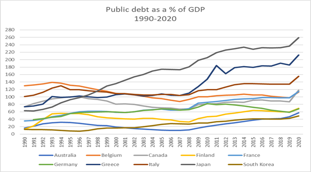
Source: Data taken from Knoema.
Looking at our graph 1, we can see that over the last 30 years the debt ratio of these countries has been increasing. Three main categories emerge. States with a debt ratio above 120% of GDP. Those with a ratio hovering around 100%, and finally a category where the ratio is below 100%. The most heavily indebted countries in our sample are Japan, with a debt-to-GDP ratio of over 250%, and Greece, with a debt-to-GDP ratio of exactly 212%. The case of Greece has become more marked since 2008, when it experienced its major economic crisis, the after-effects of which continue to this day. Italy is the third most indebted country in our sample, with public debt in excess of 150% of GDP. Alongside these countries with a high debt-to-GDP ratio, other countries such as Belgium, France and Canada have a ratio of around 100% of GDP. France, for example, has a debt-to-GDP ratio of 114% in 2020, Belgium 112% and Canada 117%. That is to say that the latter have better managed the budgetary challenges of its last years compared to the previous group, we will make an idea at the end of this work. Further in our sample, we observe a group of countries with a public debt of around 60%. Australia (57%), Germany (67%), Finland (68%) and South Korea (48%) have the lowest public debt ratios. One would tend to think that these states despite the multifaceted shocks have not experienced fiscal policies under tension. On the other hand, we can also ask ourselves whether these states are not pursuing expansionist Keynes-style policies for the recovery of the economy. Moreover, at the beginning of the 1990s, the gaps between the debt/GDP ratio were not very large, but over time the gaps have widened, as a result of the various events that have marked the history of these countries, in particular the economic crisis of 2008, which shook European countries to the core, with Greece at the epicenter. The Covid crisis from 2019 also marks a turning point in this general increase in debt. This is because economic activity was at its slowest, forcing governments to take on large numbers of people via social integration funds, putting a strain on the public finances of many countries. Other explanations would be specific to each state, such as natural disasters and poor budget consolidation policies. It should be noted, however, that most of these countries do not meet the Maastricht convergence criteria, or at least do not achieve them. Even though some countries (Finland) are very close to the threshold. We are entitled to wonder about the mechanism to be put in place to counter this surge in debt. The literature teaches us that we need to resort to the primary surplus. Is it not therefore legitimate to dwell on this?
3.1 A focus on the Primary Surplus
The measure by which an economy could overcome the snowball effect is long-term sustainability. When this is invoked, its exact specification is not defined, as many expressions are associated with it. Dietsch and Garnier (1989), analysing sustainability, propose the intertemporal budget constraint, which is the sum of budget balances over time. The aim is to show that a sustainable economy is one that respects this constraint, thereby avoiding a burden on future generations. (Martner and Tromben 2004), will refer to solvency. To demonstrate that sustainability refers to long-term solvency. Further, (Nerlich and Carolin 2018), see the sustainability of public finances as a set of rules relating to public expenditure and revenue, so that they can be maintained under predictable conditions. In other words, revenue should be able to cover expenditure so that there is no deficit at the end of each financial year. (Boissinot et al. 2004), go on to argue that a sustainable fiscal policy is one that can be pursued over the long term without leading to excessive debt accumulation. In other words, a level of debt that cannot be covered by future budget surpluses. Budget surpluses here refer to the primary surpluses that must be generated to at least stabilize debt. This is supported by (Mottoul 2008) and (Bogaert 2010), who go further by discussing the required primary surplus, which is the condition that stabilizes or causes debt to explode. In our analysis we will focus on the primary surplus.
The explosion in public debt and deficit has been analysed with the help of a number of authors. (Bogaert 2010), (Dietsch and Garnier 1989), (Fincke and Greiner 2011), (Bohn 1989) and (Neaime 2015) have analysed the process of debt accumulation from which the snowball effect derives. We know that the debt (B) is equal to the sum of the deficit (D) and the debt of the previous year. The basic relationship is similar to the following:
![]() (1)
(1)
By expressing this accounting identity as a proportion of GDP Y, we obtain the debt ratio formula, where g is the GDP growth rate.
![]() (2)
(2)
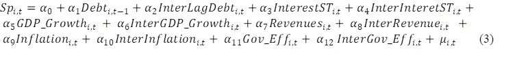
By replacing the deficit by its breakdown between the primary surplus sp and interest charges rB, and using the real interest rate r, we have successively:
![]() (3)
(3)
By transforming it, we have :
![]() (4)
(4)
![]() (5)
(5)
From the last expression, we can determine the level of primary surplus 'required'(sp*) to stabilise the debt ratio, from which (Bogaert 2010), (Martner and Tromben 2004) and Mottoul (2008), drew inspiration.
![]() (6)
(6)
![]() (7)
(7)
This shows that the snowball effect depends on the stock of debt from the previous year, the GDP growth rate, the interest rate and the primary surplus. If the real interest rate (r) exceeds the GDP growth rate (g), the level of debt will increase considerably, due to the burden of debt. If (r) is less than (g), then the government can run a primary deficit without putting upward pressure on the debt-to-GDP ratio. If r = g, the debt is stabilised (Van Parys et al. 2019), Vratislav (2009). However, given that GDP growth does not necessarily reduce debt, it follows that the interest charge is always likely to increase. It is therefore necessary to work on the primary surplus, which is the main adjustment tool in order to stabilise or at least reduce the level of debt. Using data from Knoema's websites, we have produced a graph showing the primary surpluses/deficits of 10 OECD countries. These 10 countries are chosen at random, as a chart with 33 countries would be difficult to manage.
Graph 2: Primary surplus/deficit for selected countries 1990-2020
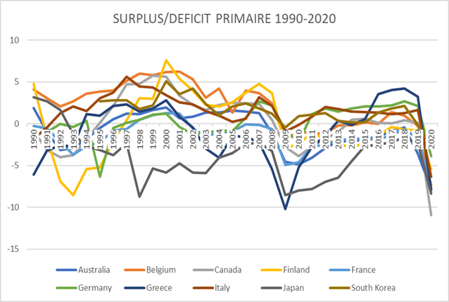
Source: Data taken from Knoema.
From graph 2, we can see that in the selected sample, no state has maintained this consistently positive balance. This is certainly due to the various difficulties encountered during the period studied. Broadly speaking, 3 periods can be identified: the first is the period from 1990 to 1996, when the primary balance declined; this can be explained by the increase in the debt-to-GDP ratio, which several states actually experienced and whose debt charges were considerable. After this period, budget balances began to rise again, remaining positive until 2008 following the economic recession. In general, however, the trend is positive. Even if there may from time to time be negative budget balances in some economies. This can be explained by the fact that many economies have been working to reduce, or at least slow down, the debt-to-GDP ratio as a result of the Solidarity and Growth Pact. Interest charges accompanied this reduction, and governments were able to build up some reserves until 2008. With the crisis of 2008, most states experienced a decline in their primary balance, due to the contagion effect of the economic crisis and its budgetary challenges. Greece is the hardest hit, with a primary balance deficit in excess of 10% of GDP. From 2019 onwards, we also see primary deficits picking up again, following the covid crisis which emerged from 2019 onwards.
4. Empirical Analysis Focusing on Public Debt
As specified above, the purpose of our research is to examine whether a debt threshold of 60% of GDP is a good measure for countering the impact of the snowball effect, in light of the Maastricht criteria. Admittedly, not all OECD countries are in Europe, but the problems of runaway debt concern all states. This is why we have chosen to conduct our analysis using this criteria.
4.1 Analysis of Descriptive Statistics
Taking the equations proposed in the theoretical analysis, we can clearly see that the determinants of the snowball effect are: the public debt ratio, the primary surplus/deficit, the GDP growth rate and the real interest rate. Our data is drawn from several sources (OECD statistics, Knoema, World Governance indicators). The descriptive statistics for our various variables are given in the table below.
Table 1: Descriptive statistics
| Obs | Mean | St. deviation | Min | Max | |
| primary surplus/deficit | 927 | -.3733646 | 3.734.601 | -29.896 | 15.826 |
| public debt | 940 | 6.184.604 | 3.972.464 | 3.765 | 259.433 |
| Budget deficit | 943 | -2.280.944 | 4.243.133 | -32.119 | 18.638 |
| GDP growth | 972 | 2.369.826 | 3.232.951 | -1.483.861 | 2.283.723 |
| Public revenue | 969 | 416.777 | 7.428.967 | 2.234.996 | 5.920.775 |
| Public expenditure | 969 | 4.396.903 | 7.733.242 | 2.048.649 | 6.793.825 |
| Short-term interest rates | 971 | 4.297.892 | 4.950.146 | -.8191667 | 45.475 |
| Long-term interest rates | 877 | 4.439.277 | 2.965.109 | -.5238333 | 28.79 |
| Inflation | 940 | 3.555.052 | 1.900.168 | -1.692.643 | 5.678.788 |
| Trade balance | 959 | .0918665 | 5.313.119 | -230.619 | 1.645.809 |
| Governance effectiveness | 704 | 1.367.346 | .4932047 | .0986325 | 2.347.191 |
| Rule of law | 726 | 1.333.715 | .5080571 | .0490841 | 2.124.782 |
From Table 1, we can see that our data are fairly stable overall. The governance variables have a smaller sample than the others, since the data for the 1990s could not be found in the database we used. We observe that our dependent variable, the primary surplus/deficit, has a negative mean over the entire period. This is evidence that the countries in our sample have had difficulty generating budget surpluses as a result of the various crises experienced during the period under study. The public debt-to-GDP ratio also averages 61.84%, a sign that the Maastricht agreements are hardly applicable in this context.
4.2 Basic Model and Data Analysis
Our data cover the period 1990-2020. The choice of this time period aims to analyse the snowball effect over two centuries, particularly in the 1980s and 1990s, when the phenomenon was first mentioned. Of the 37 countries that make up the OECD, we worked on 33 of them. The following countries: Mexico, Chile, Turkey and Costa Rica, presented data that was not always stable and sometimes unavailable. Our variables are essentially derived from the theoretical analysis presented above. These are the public debt-to-GDP ratio, the primary surplus, the GDP growth rate, and the real interest rate. In addition, other variables of fiscal policy are also included, such as public revenue and public expenditure. Alongside these basic variables, in order to stabilize our model, we have inserted economic and governance variables. The economic variables include inflation and the trade balance. The governance variables are government effectiveness and the rule of law. Our panel data are analyzed using the OLS method. The (Bohn 1998), model is our reference model. It analyses the systematic relationship between the debt-to-GDP ratio and the primary surplus. It also includes other control variables, in order to analyze the indebtedness of the United States of America over the period 1960-2000. His model suggests that the debt ratio is strongly correlated with the primary surplus, and he shows that the primary surplus required to stabilize the debt depends on the stock of debt in the previous year. This idea is reinforced by (Vratislav 2009), who analyses the same effect in 10 post-socialist EU countries. After using ordinary least squares (OLS), his conclusion is similar to that of (Bohn 1998). Our model is as follows.

Where sp is the primary surplus/deficit to GDP, ![]() is the coefficient of lag of the debt,
is the coefficient of lag of the debt, ![]() is the short-term interest rate coefficient,
is the short-term interest rate coefficient, ![]() is the GDP growth rate coefficient,
is the GDP growth rate coefficient, ![]() is the coefficient of government revenue as a percentage of GDP.
is the coefficient of government revenue as a percentage of GDP. ![]() is the coefficient of inflation in annual growth,
is the coefficient of inflation in annual growth, ![]() is the government efficiency coefficient and μ is relative to the other determinants of the primary surplus. Further, one might ask why not include public spending. It is likely that the inclusion of both public revenue and expenditure could generate a problem of multicollinearity. In principle, both would have the same influence on the model. The other economic and governance variables come from our inspiration, since we believe that fiscal policy cannot move if the economic fabric is failing or if public governance is obsolete. Our regression is based on OLS with fixed effects. After a Hausman test, we focus on a regression with fixed effects. In addition, robust standard error tests are proposed to address potential concerns about heteroskedasticity and multicollinearity. In his model, (Bohn 1998), finds that the coefficient of the lag of the debt is positively correlated with the primary surplus and thus explains the fact that a high debt in year N-1 determines a high primary surplus to be generated in year N. The results of our analysis are given in the following lines.
is the government efficiency coefficient and μ is relative to the other determinants of the primary surplus. Further, one might ask why not include public spending. It is likely that the inclusion of both public revenue and expenditure could generate a problem of multicollinearity. In principle, both would have the same influence on the model. The other economic and governance variables come from our inspiration, since we believe that fiscal policy cannot move if the economic fabric is failing or if public governance is obsolete. Our regression is based on OLS with fixed effects. After a Hausman test, we focus on a regression with fixed effects. In addition, robust standard error tests are proposed to address potential concerns about heteroskedasticity and multicollinearity. In his model, (Bohn 1998), finds that the coefficient of the lag of the debt is positively correlated with the primary surplus and thus explains the fact that a high debt in year N-1 determines a high primary surplus to be generated in year N. The results of our analysis are given in the following lines.
4.3 Empirical Results
The results of our model are presented in Table 2 below. Regression 1 is our basic model. The other regressions are used to test the robustness of our model and also allow us to better define our problem. Our regressions are carried out with the standard robustness of errors, which is achieved using the r command in Stata. Stata is our working software.
Table 2: Basic model regression
| Reg.1 | Reg.2 | Reg.3 | Reg.4 | Reg.5 | Reg.6 | Reg.7 | Reg.8 | Reg.9 | |
| LagDebt | 0.00546*** | 0.00688*** | -0.00575** | 0.00263 | 0.00488** | 0.00460** | 0.00454** | 0.00757*** | 0.00639*** |
| (0.00173) | (0.00168) | (0.00273) | (0.00207) | (0.00189) | (0.00175) | (0.00207) | (0.00223) | (0.00210) | |
| Interet_ST | 0.216*** | 0.269*** | 0.231*** | 0.219*** | 0.224*** | 0.223*** | 0.187** | 0.224*** | |
| (0.0688) | (0.0657) | (0.0628) | (0.0691) | (0.0679) | (0.0705) | (0.0691) | (0.0688) | ||
| GDP_Growth | 0.351*** | 0.392*** | 0.170*** | 0.399*** | 0.324*** | 0.324*** | 0.326*** | 0.290*** | 0.320*** |
| (0.0476) | (0.0502) | (0.0477) | (0.0500) | (0.0397) | (0.0397) | (0.0397) | (0.0409) | (0.0397) | |
| Public_Renenue | 0.192*** | 0.209*** | 0.163*** | 0.202*** | 0.199*** | 0.201*** | 0.185*** | 0.207*** | |
| (0.0246) | (0.0245) | (0.0200) | (0.0248) | (0.0263) | (0.0246) | (0.0266) | (0.0255) | ||
| Inflation | -0.182** | -0.0303 | -0.171 | -0.218** | -0.220** | -0.218** | -0.234** | -0.231** | |
| (0.0831) | (0.140) | (0.104) | (0.0848) | (0.0846) | (0.0852) | (0.0863) | (0.0909) | ||
| GOV_Eff | 1.173*** | 1.147*** | 1.975*** | 0.368 | |||||
| (0.320) | (0.352) | (0.350) | (0.425) | ||||||
| Interest_LT | 0.0222 | ||||||||
| (0.153) | |||||||||
| Public_Expenditure | -0.0549** | ||||||||
| (0.0261) | |||||||||
| Trade_Balance | 0.226*** | ||||||||
| (0.0361) | |||||||||
| Rule_Law | 0.793** | 0.799** | 0.771** | 0.872** | 0.900** | ||||
| (0.335) | (0.342) | (0.351) | (0.331) | (0.337) | |||||
| Belgium | 0.458 | ||||||||
| (0.515) | |||||||||
| Germany | 0.543 | ||||||||
| (0.426) | |||||||||
| Japan | -2.789*** | ||||||||
| (0.545) | |||||||||
| Latvia | 1.386*** | ||||||||
| (0.289) | |||||||||
| Constant | -11.39*** | -12.11*** | -1.082 | -9.526*** | -11.07*** | -10.96*** | -11.01*** | -10.36*** | -11.54*** |
| (1.038) | (1.083) | (1.293) | (0.985) | (1.078) | (1.094) | (1.094) | (1.105) | (1.125) | |
| Observations | 664 | 626 | 664 | 662 | 686 | 686 | 686 | 686 | 686 |
| R_Square | 0.247 | 0.252 | 0.122 | 0.338 | 0.234 | 0.235 | 0.235 | 0.253 | 0.239 |
| Number_Years | 22 | 22 | 22 | 22 | 22 | 22 | 22 | 22 | 22 |
Note: T-stat in brackets; ***, **, * indicate significance at the 1%, 5% and 10% thresholds respectively.
From our table 2 and in regression 1, we note that the ![]() coefficient is significant at the 1% threshold. This is quantitatively reasonable and in line with the aforementioned literature. The coefficient of 0.00173 means that a marginal increase in debt of 1% requires a primary surplus of 0.00173% the following year. This is in line with the studies by (Bohn 1998) and (Vratislav 2009). The
coefficient is significant at the 1% threshold. This is quantitatively reasonable and in line with the aforementioned literature. The coefficient of 0.00173 means that a marginal increase in debt of 1% requires a primary surplus of 0.00173% the following year. This is in line with the studies by (Bohn 1998) and (Vratislav 2009). The ![]() coefficient relating to the short-term interest rate is significantly positive at the 1% threshold, demonstrating that its impact on the primary surplus/deficit is no longer in doubt. A high interest rate increases the state's financial burden in the face of a substantial debt and requires the government to generate a considerable primary surplus in order to cope with the surge in public debt and , ipso facto, the snowball effect should it occur. The
coefficient relating to the short-term interest rate is significantly positive at the 1% threshold, demonstrating that its impact on the primary surplus/deficit is no longer in doubt. A high interest rate increases the state's financial burden in the face of a substantial debt and requires the government to generate a considerable primary surplus in order to cope with the surge in public debt and , ipso facto, the snowball effect should it occur. The ![]() coefficient concerning GDP growth in regression 1 is significant at the 1% level. This translates into the fact that the higher the growth rate of the economy, the easier it is for the primary surplus to increase, making it possible to meet debt charges and reduce the snowball effect. The same effect occurs with the
coefficient concerning GDP growth in regression 1 is significant at the 1% level. This translates into the fact that the higher the growth rate of the economy, the easier it is for the primary surplus to increase, making it possible to meet debt charges and reduce the snowball effect. The same effect occurs with the ![]() coefficient relating to public revenue. Here we note a positive significance, which implies that the primary surplus is increased when public revenues increase. This helps to improve it in a situation of weak economic growth. The
coefficient relating to public revenue. Here we note a positive significance, which implies that the primary surplus is increased when public revenues increase. This helps to improve it in a situation of weak economic growth. The ![]() coefficient relating to inflation is negatively significant at the 5% level. This is surprising, given that we would have expected the opposite effect. In any case, we believe that this could be an avenue for further research. The
coefficient relating to inflation is negatively significant at the 5% level. This is surprising, given that we would have expected the opposite effect. In any case, we believe that this could be an avenue for further research. The ![]() coefficient is significantly positive at the 1% threshold. It relates to government effectiveness, i.e. the perception of the quality of public services, the quality of the civil service and its degree of independence from political pressures, the quality of policy formulation and implementation, and the credibility of the government's commitment to its policies. In our view, this is correct insofar as a state that advocates government efficiency easily implements its public policies, including the budget.
coefficient is significantly positive at the 1% threshold. It relates to government effectiveness, i.e. the perception of the quality of public services, the quality of the civil service and its degree of independence from political pressures, the quality of policy formulation and implementation, and the credibility of the government's commitment to its policies. In our view, this is correct insofar as a state that advocates government efficiency easily implements its public policies, including the budget.
In regression 2 we inserted the long-term interest rate variable. This did not prove to be significant. Does this mean that a long-term interest rate has less effect on the primary budget balance? This remains to be verified. As in the case of short-term interest rates, we assume that its sign is positive. In regression 3, we inserted the public spending variable. We note a negative significance at the 5% threshold. This is in line with our problem and is similar to that of public revenue, which showed positive significance. In regression 4, we inserted the trade balance variable in order to analyse its effects on fiscal policy, particularly with regard to the primary surplus/deficit. We note a positive significance at the 1% threshold, which would indicate that a positive trade balance increases government revenues, which has a positive impact on the government budget balance and ipso facto on the primary balance. In regression 5, we inserted another governance variable, the rule of law, which showed positive significance at the 5% threshold. Like government effectiveness, the rule of law reflects the extent to which citizens trust and respect social rules. In particular, the quality of the enforcement of contracts, property rights, the police and the courts, as well as the likelihood of crime and violence. In our sample, it has a positive impact on fiscal policy. In regressions 6, 7, 8 and 9, we wanted to show the specific aspects to each country by isolating them from the other countries. We note that over the period 1990 and 2020, certain countries such as Belgium and Germany would not have had a significant influence on the budget balance. Japan would have had a negative impact on its primary balance, while Latvia would have had a positive impact on its primary balance. Is it because it's a small country among the big ones, or is its fiscal policy more robust? This is more of a research question. Our model is stable overall, but does not answer our problem. Following this, we are setting up another model to determine whether a debt threshold of 60% is a robust measure for limiting the snowball effect.
4.4 Debt Analysis at 60% Threshold
Our objective, as outlined above, is to verify whether a debt threshold of 60% is a good measure to avoid the snowball effect. Following (De Grauwe & Ji 2015), we introduce a binary variable that simulates in the regression a debt rate below and above 60% of GDP. This takes the value 1 if this rate is lower, and 0 when it is higher. Our equation takes the following form.

Where ![]() is the coefficient of the binary variable introduced into the regression to capture the effects of the simulation. The other coefficients are those used above in model 1. Also, in order to better process our model, we are entitled to use other variables that could better help us in the interpretation. To this end, and still following (De Grauwe & Ji 2015), we introduce interaction variables to verify our observations. Here, our binary variable of debt interacts with the other variables of model 1 which allows us to have the following model:
is the coefficient of the binary variable introduced into the regression to capture the effects of the simulation. The other coefficients are those used above in model 1. Also, in order to better process our model, we are entitled to use other variables that could better help us in the interpretation. To this end, and still following (De Grauwe & Ji 2015), we introduce interaction variables to verify our observations. Here, our binary variable of debt interacts with the other variables of model 1 which allows us to have the following model:
Where ![]() ,
, ![]() ,
, ![]() ,
, ![]() ,
, ![]() ,
, ![]() , are respectively the coefficients of the interaction variables with the binary variable on the other variables: debt, interest rate, GDP growth rate, government revenue, inflation and government efficiency. The results of our two models are given in the following table:
, are respectively the coefficients of the interaction variables with the binary variable on the other variables: debt, interest rate, GDP growth rate, government revenue, inflation and government efficiency. The results of our two models are given in the following table:
Table 3: Specific model regression
| Reg.1 | Reg.2 | |
| LagDette | 0.00877*** | -0.000615 |
| (0.00188) | (0.00363) | |
| InterLagDebt | 0.0118** | |
| (0.00479) | ||
| Interet_ST | 0.199** | 0.224* |
| (0.0710) | (0.115) | |
| InterInteret_ST | -0.0428 | |
| (0.105) | ||
| GDP_Growth | 0.301*** | 0.425*** |
| (0.0441) | (0.0664) | |
| InterGDP_Growth | -0.140** | |
| (0.0543) | ||
| Revenue | 0.201*** | 0.220*** |
| (0.0253) | (0.0256) | |
| InterRevenue | -0.0720*** | |
| (0.0153) | ||
| Inflation | -0.187** | -0.108 |
| (0.0899) | (0.191) | |
| InterInflation | -0.0574 | |
| (0.214) | ||
| GOV_Eff | 1.167*** | -0.612 |
| (0.322) | (0.374) | |
| InterGov_Eff | 2.797*** | |
| (0.357) | ||
| Bin_Debt | 1.259*** | |
| (0.216) | ||
| Constant | -12.48*** | -10.53*** |
| (1.145) | (1.072) | |
| Observations | 664 | 664 |
| R_Square | 0.278 | 0.315 |
| Number of years | 22 | 22 |
Note: T-stat in brackets ; ***, **, * indicate significance at the 1%, 5% et 10% thresholds respectively.
From table 3, regression 1, which is the one relating to our model 2, presents us with results that we can examine. Our main variable (binary) is significant at the 1% threshold. In any case, this would mean that a debt ratio of less than 60% improves the primary surplus by 0.21%. This is positive for fiscal policy, as every penny saved constitutes a financing reserve for other projects, as we know our economic system needs them. We can therefore say that a debt level of 60% of GDP improves the primary surplus, which is the main tool for stabilizing or even reducing the snowball effect.
In regression 2, we can draw a number of conclusions, which we will limit to commenting on a few variables. If we take the lag of the debt and its interaction variable in our regression, we note that for a debt ratio of less than 60%, the primary surplus that a state must generate is considerably reduced. Since the coefficients 0.00363 and 0.00479 mean that in such a situation, the government would have to generate a primary surplus of 0.00116 (-0.00363 +0.00479). This would help to reduce the pressure on public finances. Thanks to this difference, the economy is positively impacted. We also note that the effect of the public revenue variable and its interaction variable is similar. As we have shown above, an increase in revenue improves the primary surplus, which leads to an improvement in fiscal policy. In our case, in a situation of debt at the 60% threshold, the primary surplus would improve by 0.0103 (0.0256 - 0.0153). When we look at GDP growth, we see that the same effect stands out, as GDP growth improves by 0.0121 (0.0664-0.0543). We can explain this result by the fact that when an economy has too much debt, recovery efforts are difficult insofar as the funds that could have been used for investment to revive the economy are diverted towards servicing the debt. With a reduction in debt, there is renewed hope of growth. We note that in the case of the short-term interest rate, the effect is similar to that of the other variables mentioned above. The governance and economic variables will not be commented on insofar as they were used to stabilize our models. All of which goes to show that governments would do well to reduce debt levels, as they are a real brake on the emancipation of public finances in all nations. Reducing debt has several benefits: it allows the sums earmarked for interest charges to be made available to other sectors of the economy, thus avoiding the crowding-out effect. It also allows the economy to generate more primary surpluses, which are made available to the economy to deal with crises (health, security, etc.) of all kinds. Finally, reducing debt gives governments a degree of credibility when it comes to contracting international debt.
5. Budget Deficit Analysis
The budget deficit is one of the criteria adopted by Europe through Maastricht to contain soaring budget deficits and debt. A government has a budget deficit when its spending in a given year exceeds its tax revenues and income, (Stiglitz et al. 2018). The budget deficit is, in a way, the financing requirement of a state or organization that must be financed by debt during a financial year. The deficit is calculated using the following equation:
![]() , where B is the debt and D the deficit.
, where B is the debt and D the deficit.
From equation, we can easily derive the budget deficit . The following graph gives us an idea of the budget deficits of 10 countries taken from our sample of OECD countries as a percentage of GDP. It should be remembered that we have chosen 10 countries, as a graph with 33 countries would be difficult to manage.
Graph 3: Budget deficits of some OECD countries
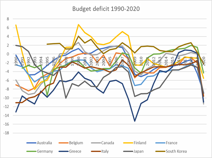
Data taken from Knoema.Graph produced by us
Graph 3 shows that budget deficits are not stationary. Depending on the circumstances (economic crisis, war, energy crisis, etc.), deficits can be huge and sometimes stable. For all the countries in our sample, the peak was in 2009, at the height of the economic crisis. Greece and Japan were the hardest hit, with deficits of 15.27% and 9.6% of GDP respectively. South Korea seems to be coping better than the other countries. It has achieved a degree of stability in its borrowing requirement, which in our sample is positive over almost the entire period under review. These deficits are sometimes below and sometimes above 3% of GDP. As required by Maastricht, with this threshold can we hope to see the snowball effect avoided in the economies of the OECD countries?
5.1. Quantitative Analysis
4.1.1. Model
The aim of our analysis is to check whether, below a threshold of 3%, fiscal policy tends towards sustainability, which tends towards the intertemporal budget constraint. To do this we use data from the same countries as presented above. Using the OLS method, we regress the primary surplus/deficit as the dependent variable on the other explanatory variables. Our key independent variable is the budget deficit. As this model has no precedent, as was the case with public debt, we propose to include it as an innovation. Our regression equation is as follows:

Where ![]() is the budget deficit coefficient,
is the budget deficit coefficient, ![]() is the coefficient of GDP growth lag,
is the coefficient of GDP growth lag, ![]() is the coefficient lag of public expenditure,
is the coefficient lag of public expenditure, ![]() is the short-term interest rate coefficient,
is the short-term interest rate coefficient, ![]() is the lag coefficient of inflation and
is the lag coefficient of inflation and ![]() is the trade balance coefficient.
is the trade balance coefficient.
5.1.2. Results
The results are shown in the table below:
Table 4: Regression with the budget deficit
| Reg.1 | Reg.2 | Reg.3 | |
| Deficit | 0.770*** | 0.767*** | 0.811*** |
| (0.0214) | (0.0215) | (0.0215) | |
| LagGdpGrowth | 0.0769** | 0.0551* | 0.0887** |
| (0.0336) | (0.0315) | (0.0338) | |
| LagExpenditure | 0.0442*** | 0.0658*** | |
| (0.00664) | (0.00754) | ||
| Interest_ST | 0.0431* | 0.0400 | |
| (0.0241) | (0.0240) | ||
| LagInflation | -0.0572* | -0.0494 | -0.0855*** |
| (0.0314) | (0.0307) | (0.0305) | |
| Trade_Balance | -0.0291* | -0.0294* | -0.0462** |
| (0.0159) | (0.0155) | (0.0220) | |
| LagRevenue | 0.0340*** | ||
| (0.00502) | |||
| Interest_LT | 0.227*** | ||
| (0.0686) | |||
| Constant | -0.900** | -0.343 | -2.447*** |
| (0.328) | (0.249) | (0.453) | |
| Observations | 820 | 820 | 765 |
| R-square | 0.767 | 0.764 | 0.803 |
| Number of years | 31 | 31 | 31 |
Note: T-stat in brackets ; ***, **, * indicate significance at the 1%, 5% et 10% thresholds respectively.
From Table 4, we can see that our model is fairly heterogeneous in terms of results. We will comment on some of the results. Regression 1 in this framework is our basic model. Our key variable (budget deficit) is significant at the 1% level. The ![]() coefficient would mean that for a 1% increase in the deficit, it increases the primary surplus to be generated to cover the government's financing needs by 0.02%. This is in line with our expectations. Indeed, as we have noted in graph 3, in years such as 2009, when most OECD countries experienced the economic crisis and very high deficits, economic and structural sacrifices had to be made to postpone the effects of the crisis and get the economies moving again. One of the levers, of course, was to increase the primary balance in the face of economies experiencing very little economic growth. The
coefficient would mean that for a 1% increase in the deficit, it increases the primary surplus to be generated to cover the government's financing needs by 0.02%. This is in line with our expectations. Indeed, as we have noted in graph 3, in years such as 2009, when most OECD countries experienced the economic crisis and very high deficits, economic and structural sacrifices had to be made to postpone the effects of the crisis and get the economies moving again. One of the levers, of course, was to increase the primary balance in the face of economies experiencing very little economic growth. The ![]() coefficient is significant at the 5% level. Although moderately significant, GDP growth improves the primary surplus. If GDP growth increases by 1%, the primary surplus improves by 0.033%. the
coefficient is significant at the 5% level. Although moderately significant, GDP growth improves the primary surplus. If GDP growth increases by 1%, the primary surplus improves by 0.033%. the ![]() coefficient shows a positive sign compared to the public debt model. Although significant at 1%, we note that it positively impacts the surplus/deficit. What is a curiosity one would have expected to have a negative sign. This nevertheless remains avenues for further reflection. The
coefficient shows a positive sign compared to the public debt model. Although significant at 1%, we note that it positively impacts the surplus/deficit. What is a curiosity one would have expected to have a negative sign. This nevertheless remains avenues for further reflection. The ![]() coefficient, on the other hand, is weakly significant, recording a significance level of 10% at the confidentiality threshold. Nevertheless, it remains positive, showing its impact on fiscal policy and therefore on the budget balance. The
coefficient, on the other hand, is weakly significant, recording a significance level of 10% at the confidentiality threshold. Nevertheless, it remains positive, showing its impact on fiscal policy and therefore on the budget balance. The ![]() and
and ![]() coefficients are also weakly significant (10%). In reality, these two variables serve as control variables, allowing us to test the robustness of the model. In regression 2, we have inserted the public revenue lag in order to check whether the same result can be observed in comparison with public expenditure in the previous regression. We also note a significance at the 1% confidentiality threshold. This indicates that our model is stable overall. In regression 3, we have included the long-term interest rate, since in our basic model it also reveals a positive significance, this time at the 1% confidentiality threshold. In reality, the idea remains the same: an increase in interest rates implies major efforts in terms of the primary surplus in order to keep fiscal policy stable. At this point, we might ask what would happen if the budget deficit complied with the Maastricht criteria.
coefficients are also weakly significant (10%). In reality, these two variables serve as control variables, allowing us to test the robustness of the model. In regression 2, we have inserted the public revenue lag in order to check whether the same result can be observed in comparison with public expenditure in the previous regression. We also note a significance at the 1% confidentiality threshold. This indicates that our model is stable overall. In regression 3, we have included the long-term interest rate, since in our basic model it also reveals a positive significance, this time at the 1% confidentiality threshold. In reality, the idea remains the same: an increase in interest rates implies major efforts in terms of the primary surplus in order to keep fiscal policy stable. At this point, we might ask what would happen if the budget deficit complied with the Maastricht criteria.
5.2. Analysis of the Deficit at 3% of GDP
5.2.1. Model
To do this we introduce a binary variable which simulates the budget deficit when it is less than 3% of GDP. This variable takes the value 1 if the deficit is greater than or equal to -3 and 0 if it is less than -3. Our regression equation takes the following form:

Where ![]() , is the coefficient of the binary variable we introduced. Also, in the interests of better understanding, we interacted our binary variable with the other variables in our regression in order to interpret its impact on our results. Our model is as follows:
, is the coefficient of the binary variable we introduced. Also, in the interests of better understanding, we interacted our binary variable with the other variables in our regression in order to interpret its impact on our results. Our model is as follows:
5.2.2. Results
The results of our regressions are given in the following table:
Table 5: Robustness regression
| Reg.1 | Reg.2 | Reg.3 | Reg.4 | |
| Deficit | 0.800*** | 1.003*** | 0.958*** | 1.006*** |
| (0.0248) | (0.0985) | (0.0846) | (0.0986) | |
| InterDeficit | -0.224** | -0.110 | -0.231** | |
| (0.0942) | (0.0775) | (0.0940) | ||
| LagGDP_Growth | 0.0743** | -0.0544 | -0.0351 | -0.0683 |
| (0.0345) | (0.0924) | (0.0952) | (0.0970) | |
| InterGDP_Growth | 0.147 | 0.133 | 0.138 | |
| (0.0954) | (0.100) | (0.0995) | ||
| LagPub_Exp | 0.0417*** | 0.0416* | 0.0473** | |
| (0.00651) | (0.0220) | (0.0198) | ||
| InterExpen | 0.00399 | 0.0186 | ||
| (0.0182) | (0.0148) | |||
| Interest_ST | 0.0492** | -0.155 | -0.164 | |
| (0.0235) | (0.118) | (0.134) | ||
| InterInterest_ST | 0.227* | 0.228 | ||
| (0.122) | (0.138) | |||
| LagInflation | -0.0532* | -0.0516* | -0.0727*** | -0.0430 |
| (0.0280) | (0.0267) | (0.0251) | (0.0264) | |
| InterInflation | -0.0454 | -0.105* | -0.0382 | |
| (0.0447) | (0.0572) | (0.0439) | ||
| Trade_Bal | -0.0282* | -0.145** | -0.101 | -0.161** |
| (0.0152) | (0.0663) | (0.0623) | (0.0647) | |
| InterTrade_Bal | 0.121* | 0.0496 | 0.139** | |
| (0.0684) | (0.0564) | (0.0667) | ||
| BinaryDeficit | 0.799** | |||
| (0.330) | ||||
| Interest_LT | 0.122 | |||
| (0.134) | ||||
| InterInterest_LT | 0.137 | |||
| (0.120) | ||||
| LagPUB_Rev | 0.0295 | |||
| (0.0236) | ||||
| InterPUB_Rev | 0.00401 | |||
| (0.0212) | ||||
| Constant | -1.497*** | -0.950** | -2.266*** | -0.308 |
| (0.386) | (0.405) | (0.565) | (0.339) | |
| Observations | 820 | 804 | 750 | 804 |
| R-square | 0.769 | 0.775 | 0.812 | 0.772 |
| Number of Years | 31 | 31 | 31 | 31 |
Note: T-stat in brackets ; ***, **, * indicate significance at the 1%, 5% et 10% thresholds respectively.
The results of our regressions are interesting. In regression 1, we find that our binary variable is significant at the 1% confidentiality threshold. This is sufficient evidence that, if an economy remains below this threshold over the long term, it will tend towards a balanced budget, which is similar to the intertemporal budget constraint mentioned above. So an economy that keeps its budget deficit below 3% of GDP has the advantage that its debt does not grow, or at least grows very little. And if it does grow very little, it does not lead to high debt charges. As the debt burden is lower, it keeps the economy away from the snowball effect. With the snowball effect behind us, the funds allocated to servicing the debt are freed up to fuel other economic sectors. The other important aspect is that the primary surplus is increasing. The increase in the primary surplus means that at times of crisis, the economy is not severely impacted. This was the case in Italy when the crisis hit in 2009. Despite its high level of debt, it was not affected to the same extent as Greece, thanks to the primary surpluses generated in previous years.
In regression 2, where we have made our different variables interact with the binary variable, we note that in the case of the ![]() and
and ![]() coefficients, a budget deficit at the threshold of 3% of GDP leads to less effort being made by fiscal policy with regard to the primary surplus. In fact, in this situation the primary surplus would gain 0.0043 (0.0985 - 0.0942) effort point as a budgetary sacrifice in order to stabilize the soaring budget deficit and also the debt. The same can be observed with the other variables. Whether it is GDP growth, short- or long-term interest rates, public expenditure and revenue, or economic variables, we note that a budget deficit at the 3% threshold shows some stability of the other variables in relation to the primary surplus/deficit. It is therefore worthwhile for governments to work towards reducing debt and deficits by combating phenomena capable of undermining fiscal policy, in particular by rigorously consolidating public finances.In addition, governments would do well to focus public spending on sectors with strong economic potential and reduce funding for sectors that are not conducive to economic development.
coefficients, a budget deficit at the threshold of 3% of GDP leads to less effort being made by fiscal policy with regard to the primary surplus. In fact, in this situation the primary surplus would gain 0.0043 (0.0985 - 0.0942) effort point as a budgetary sacrifice in order to stabilize the soaring budget deficit and also the debt. The same can be observed with the other variables. Whether it is GDP growth, short- or long-term interest rates, public expenditure and revenue, or economic variables, we note that a budget deficit at the 3% threshold shows some stability of the other variables in relation to the primary surplus/deficit. It is therefore worthwhile for governments to work towards reducing debt and deficits by combating phenomena capable of undermining fiscal policy, in particular by rigorously consolidating public finances.In addition, governments would do well to focus public spending on sectors with strong economic potential and reduce funding for sectors that are not conducive to economic development.
Compliance with the Maastricht criteria is, in absolute terms, the ideal for any economy wishing to emancipate itself from debt, but the reality is that no economy is immune to economic conditions (unemployment, among others), which means that it has to adapt accordingly. Further on, if the debt were to be reduced, wouldn't social charges in a Western context characterized by an ageing population be the other side of the iceberg, i.e. another reason why public spending would be under serious threat?
5. Conclusion
At the end of our analysis, we analyzed the snowball effect. In order to analyze this phenomenon, we wanted to answer the question of whether the Maastricht convergence criteria, i.e. a public debt threshold of 60% of GDP and a deficit threshold of 3% of GDP are good measure to avoid the snowball effect. After empirical analysis, we have observed that below these thresholds, the primary surplus required to stabilize soaring debt is reduced, putting less pressure on fiscal policy. However, if the debt-to-GDP ratio were to fall, this would not mean that the economy would be spared, as debt charges could prove even more threatening, especially if interest rates were to rise. Nowadays, states strive to have low interest rates in order not to face the burden on the huge debt, which allows them to avoid the snowball effect. Since the debt-to-GDP ratio of states tends to remain high or very high for many OECD states. And, due to the fact that this rate is still high is preventing states from emancipating themselves, as the dangers are so close at hand (economic conditions, social charges and multiform crises). Governments therefore need to find mechanisms to generate substantial primary surpluses in order to prevent these difficult times. This would also help to prove the credibility and solvency of these states. So when the inevitable loan situation arises, these states would be granted credit at very low rates, which would not burden them with debt.
---
Funding: This research received no funding.
Conflicts of Interest: The author declares no conflict of interest.
---
Disclaimer/Publisher’s Note: The views, statements, opinions, data and information presented in all publications belong exclusively to the respective Author/s and Contributor/s, and not to Sprint Investify, the journal, and/or the editorial team. Hence, the publisher and editors disclaim responsibility for any harm and/or injury to individuals or property arising from the ideas, methodologies, propositions, instructions, or products mentioned in this content.
References
- Baglioni, A. and Cherubini, U., 1993. Intertemporal budget constraint and public debt sustainability: the case of Italy. Applied Economics, 25, p. 275–283.
- Barro, R. J., 1979. On the determination of public debt. Journal of political economy, October, 87, pp. 940-971.
- Bogaert, H., 2010. Le retour de l’effet boule de neige. Communication à l’Institut Belge des Finances Publiques.
- Bohn, H., 1998. The behavior of U.S public debt and deficits. Quaterly Journal Of Economics, pp. 113, pp.949-963.
- Bohn, H., 2005. The sustainability of fiscal policy in the United States. Working Paper Series No. 1446. Center for Economic Studies and Ifo Institute..
- Boissinot, J; L'Angevin, C. & Monfort, B., 2004. Public debt sustainability: some results on the French case. Institut National de la Statistique et des Etudes Economiques., Issue N° G2004-10.
- Bruggeman, A. & van Nieuwenhuyze, Ch; 2013. Ampleur et dynamique de l’endettement en Belgique et dans la zone euro. BNB, Révue économique.
- Buchanan, M. J., 1957. External and Internal public debt. American economic association, 47(6), pp. 995-1000.
- Castro, G., Ricardo M. F., P. Jùlio., J. R. Maria 2015. Unpleasant debt dynamics: Can fiscal consolidations raise debt ratios? Journal of Macroeconomics, 44, pp. 276-294.
- Catrina, I.L., 2017. How to stop the snowball growth? A way for sustaining public debt over generations. HOLISTICA–Journal of Business and Public Administration, 8(2), pp.59-68.
- De Grauwe, P. &. Ji. Y., 2013. Self-fulfilling crises in the Eurozone: An empirical test. Journal of International Money and finance, 34, pp. 15-36.
- Delvaux, Y., 1990. La dette publique. Courrier hebdomadaire du CRISP, 26, pp. 1-46.
- Dietsch, M. and Garnier, O., 1989. La contrainte budgétaire intertemporelle des administrations publiques: conséquences pour l'évaluation des déficits publics. Économie & prévision, 90(4), pp.69-85.
- Fincke, B. and Greiner, A., 2011. Debt sustainability in Germany: empirical evidence for federal states. International Journal of Sustainable Economy, 3(2), pp.235-254.
- Izák, V., 2009. Primary balance, public debt and fiscal variables in postsocialist member of the european union. Prague Economics Papers.
- Martner, R. and Tromben, V., 2004. Public debt indicators in Latin American countries: snowball effect, currency mismatch and the original sin. Currency Mismatch and the Original Sin (April 1, 2004).
- Meade, E. J., 1958. Is the National Debt a Burden?. Oxford Economic Papers, New Series, 10(2), pp.163-183.
- Minsky, H.,1992. The financial instability hypothesis. The Jerome Levy Economics Institute Working paper.
- Monnier, J.-M. & B. Tinel, 2006. Endettement public et redistribution en France de 1980 à 2004. Cahiers de la maison des sciences économiques .
- Mottoul, J. M., 2008. Effet boule de neige et solde paquebot. Federale Overheidsdienst Financien – Belgie.
- Neaime, S., 2015. Sustainability of budget deficits and public debts in selected European Union countries. The Journal of Economic Asymmetries.
- Pagano, G., 2007. Les recommandations du Conseil supérieur des finances sur le coût du vieillissement. Courrier hebdomadaire, pp.5-48.
- Pagano, G., 2021. Finances publiques: la Belgique fédérale dans l'Europe. Bruxelles: Éditions de l'Université Ouverte de la Fédération Wallonie-Bruxelles.
- Reinhart, C. M. & K. S. Rogoff, 2010. Growth in a Time of Debt. American economic review 100.2, pp. 573-578.
- Requeijo, J., 2010. The Aftermath. pp. 1-16.
- Sharp, A.M., 1959. A general theory of public debt.
- Stiglitz, J.E., Lafay, J.D. and Rosengard, J., 2018. Economie du secteur public. De Boeck Supérieur.
Article Rights and License
© 2024 The Author. Published by Sprint Investify. ISSN 2359-7712. This article is licensed under a Creative Commons Attribution 4.0 International License.