Fiscal Decentralization and Government Expenditure Efficiency in Indonesia: A Malmquist Productivity Index

Keywordsefficiency fiscal decentralization government expenditure Indonesia Malmquist Productivity Index Tobit model

JEL Classification C14, C24, H11, H50

Full Article

1. Introduction

For the past two decades, Indonesia has been implementing regional autonomy since 1999. The “big bang” of regional autonomy changed a centralized government into a decentralized system, followed by the application of fiscal decentralization in 2004. It has been broadly considered that in a decentralized government system, public service performance significantly differs depending on the efficiency of the regional government delivering services (Afonso et al., 2005). After implementing fiscal decentralization, a province with good performance might become worse because of mismanagement or the lack of qualified human resources, or it might become more efficient because it has greater authority in managing local resources. The evaluation of regional government performance warrants attention if we consider that regional bureaucrats might have a greater incentive to perform not in the interest of social welfare but by wasting resources to gain private profit. In his seminal paper, Prud’homme (1995) argues that decentralization may become a danger despite its objective to bring government services closer to the people. For these related reasons, this study mainly focuses on analyzing the impact of fiscal decentralization on facilitating or hindering regional government efficiency at the provincial level in Indonesia.

Given the uniqueness of Indonesia’s socioeconomic condition, this study is ideal research that contributes to measuring regional government efficiency. This study fills a gap in existing research by incorporating a data set of input and output data to be internationally comparable with other seminal studies, such as that by Afonso et al. (2010). More importantly, it aims to assess the determinants of whether the degree of fiscal decentralization and other factors affect the performance of government efficiency. To the best of our knowledge, no previous studies in Indonesia have applied a two-stage approach to analyzing the relationship between the degree of fiscal decentralization and government expenditure efficiency. This study contributes by employing a Malmquist productivity index (MPI) approach; it calculates the efficiency scores in the first stage and assesses the impacts of nondiscretionary factors and the degree of fiscal decentralization on government efficiency in the second stage by utilizing a Tobit model.

Efforts to measure government expenditure efficiency have attracted the interest of many scholars. Mihaiu et al. (2010) performed a comparative analysis of efficiency in the public and private sectors and found difficulties in quantifying efficiency in the public sector. Some characteristics in the public sector, such as its politician-driven nature, the extent to which the interests of citizens are not reflected, complex procedures and organizations, strict regulations, poorly funding, and the suspicious attitude of citizens toward the government, cause difficulties in measuring public service outcomes. Although, by its very nature, public service is not easily measured, Afonso et al. (2010) emphasize the need for government expenditure in the development process because of the government’s roles in providing genuine public goods, confronting significant externalities resulting from the private sector, creating social institutions and establishing the rule of law to protect individuals and property.

Accordingly, this research aims to answer the following research questions. First, how large are the productivity and efficiency scores of government expenditure, particularly in infrastructure, education, health and social protection? Second, what is the relationship between the degree of fiscal decentralization and government expenditure efficiency in Indonesia’s provinces? After investigating these two research questions using a two-stage procedure, the estimation results reveal evidence that expenditure decentralization is a factor that contributes to promoting the efficiency of infrastructure, education and health expenditure; however, the degree of fiscal decentralization seems to reduce the efficiency of social protection expenditure.

This introduced is followed by four sections. The literature review elaborates a number of existing studies in this field. The data and methodology both in the first stage using the MPI and in the second stage using the Tobit model are comprehensively discussed. The following section presents the estimation results and the discussion of the results, and the last section draws conclusions.

2. Literature Review

There have been many studies that have investigated fiscal decentralization and the channel through which it affects government expenditure efficiency. A recent study by Adam et al. (2014) summarizes two benchmark channels: first, electoral control and, second, yardstick competition among local governments. According to Hindrisk and Lockwood (2009), electoral control may position decentralization to reduce the tendencies of local government officials to create rents. Local people have the power to elect good leaders and vote out bad leaders. Electoral control seems to promote government efficiency. A similar view is noted by Myerson (2006). From the yardstick competition perspective, citizens benefit when they can evaluate government performance and compare it with that of their neighboring regions (Basley and Case, 1995). Similarly, Basley and Smart (2007) point out that citizens can compare public services and regional development across regions and assess public official integrity (rent-seeking and bribing practices in public offices). Competition across jurisdictions is expected to increase government efficiency.

In addition to the advantages created fiscal decentralization, fiscal decentralization can exert a negative effect on government efficiency. In a seminal study, Prud’homme (1995) argued that fiscal decentralization may encourage pressure imposed by a local interest group on a region with a small size of jurisdiction. He emphasizes the advantage of centralized government, which notably provides better career and job opportunities for talented and highly qualified human resources. As discussed above, existing studies have reached inconclusive findings on the relationship between fiscal decentralization and public service efficiency (PSE). These varied findings may depend on the methodology used, the research scope and the study period.

A critical debate arises regarding the measure of government performance. Afonso et al. (2010) criticize economists for having a tendency to measure government activities based on budget allocations, where higher expenditures reflect higher benefits. Additionally, some authors, such as Fisman and Gati (2002), and Enikolopov and Zhuravskaya (2007), have driven the development of the quality of governance and fiscal decentralization, and they measure the quality of governance using internationally comparable outcomes such as the literacy rate and infant mortality. Socioeconomic measures are constrained to serve as a measure of governance quality; these measures do not deal with the size of government spending and the level of efficiency generated from this spending. To address this issue, a number of studies, such as Adam et al. (2014), Afonso et al. (2010), Afonso et al. (2006), have developed a direct measure of government expenditure efficiency or have mostly defined government expenditure efficiency as PSE. The PSE measure is constructed using the input and output information of the public sector, and it reflects government efficiency in delivering services and assumes that the inputs and outputs of the public sector are derived from the government production function.

A few studies have examined the efficiency of regional governments in Indonesia and its relationship with fiscal decentralization. Using a two-stage methodology consisting of data envelopment analysis (DEA) and a Tobit model, Tirtosuharto (2010) finds that the degree of fiscal decentralization is the key determinant of regional fiscal efficiency. He reveals that the expansion of a regional government’s fiscal spending has caused some degree of inefficiency due to the growing corruption and rent-seeking at the level of regional governments. In contrast, in his dissertation, Arsana (2014) assesses the growth in productivity of the Indonesian regional governments using a DEA-based MPI approach. He finds that, on average, the growth in regional productivity was more than one and that the dominant factor of growth in regional productivity was efficiency change, which was offset by technological regress.

3. Data and Methodology

3.1. Measurement of Government Expenditure Efficiency – Data

The government expenditure efficiency frontier approach remains challenging because of the scarcity of regional-level data. This study opts to adopt an MPI based on DEA. The panel data cover 26 out of 33 provinces in Indonesia in the 2004-2015 period. The start of the study period is 2004 because we intend to use the audited version of the budget realization report at the provincial level. All regional government financial data are obtained from the Ministry of Finance.

To measure the productivity index of government expenditure, this study proposes four prominent types of expenditures: infrastructure, education, health and social protection. Some studies, such as those by Afonso and Aubyn (2005, 2006) and Clements (2002), examine the public spending performance of education and health expenditure. Afonso et al. (2005) compute public sector efficiency using four outcomes: administration, education, health and public infrastructure. In contrast to existing studies, we add social protection expenditure to the other expenditures to meet some objectives. First, healthy and educated human resources are fundamental elements in development. The infrastructure in developing countries has provided evidence of the growth-enhancing factor. The infrastructure effect, for example, from the construction of roads, bridges, and ports and the provision of electricity, significantly contributes to supporting economic development by providing greater access to society. Second, the introduction of social protection expenditure is motivated by the fact that the government is the dominant actor socially responsible for lifting poor people out of poverty, redeveloping a region after a natural disaster and providing subsidies in periods of crisis. The contribution of the government with regard to both infrastructure and social protection is mandatory and significant. All four types of expenditures represent the inputs of the government in the MPI.

In the productivity measure, the efficiency of inputs is analyzed with the corresponding outputs. The MPI allows several inputs and outputs to be included in the model. In the productivity measure, the challenge is finding the best available data; hence, we follow previous studies in constructing the output data. The choice of output variables warrants a debate and further discussion. The selection is related to the degree of suitability for use as a proxy of the outcome. Following Afonso et al. (2005), the outputs for infrastructure expenditure are represented by the length of roads in a province (in km) and the supply of electricity for public facilities such as public street lighting and social facilities (per mega volt amp (MVA)). The length of roads in a province categorized as good is obtained from Statistics Indonesia (the Indonesian statistical bureau) and is measured as flow data. The electricity data are obtained from the state electricity company (a state-owned company). The other data are available from Statistics Indonesia. The outcome of education expenditure is reflected by two outputs: the number of school buildings for primary and secondary schools and the enrollment rate at the primary and secondary school levels. The number of school buildings is constructed in flow data, and the unit is the number of buildings. All outputs related to education expenditure are gathered from Statistics Indonesia. The outputs of health expenditure are indicated by three variables: life expectancy (in years), the infant mortality rate (the rate is inverted) and the number of elderly people (people over 65 years of age). Finally, social protection expenditure corresponds to two outputs: the number of poor people and the unemployment rate (inverted). For more details, the descriptive statistics are available in table (1).

Table 1. Descriptive Statistics of the Input and Output Variables – The Malmquist Productivity Index

Note: The inputs are infrastructure, education, health, and social protection expenditures. The outputs of infrastructure expenditure are the road length (good) and the electricity supply for public lighting and social facilities. The outputs of education expenditure are primary school buildings, secondary school buildings, and primary school and secondary school enrollment rates. The outputs of health expenditure are life expectancy (years) and the mortality rate. The outputs of social protection expenditure are the number of older people, poor people and the unemployment rate.

3.2. Malmquist Production Index

Many previous studies on government expenditure efficiency conduct DEA, which is a nonparametric approach, to measure the efficiency index, while some studies propose the MPI to measure the total factor productivity (TFP) of government expenditure. Both methodologies measure relative efficiency with multiple inputs and outputs in a linear manner, they make no assumption on the underlying functional form of a production function, and they allow for different units of measurements. The advantage of using the MPI is that the MPI can distinguish between changes in efficiency and changes in the production frontier, which is useful for policy purposes. TFP can be decomposed into two measurements: technical efficiency change (TEC) and technological change (TC). TEC is defined as the change in the best practice production frontier, and efficiency change includes all other types of productivity change, such as learning by doing, the diffusion of new technological knowledge, and improved managerial practice (Nishimizu and Page, 1982).

Following Färe et al. (1994), this study utilizes an MPI and input-based DEA to calculate the TFP index, which is defined as the geometric mean of two productivity indices between periods t and t+1. The MPI is one prominent method for measuring relative productivity changes over time. Compared to other frontier methodologies, the MPI presents some important properties that are useful in measuring public sector efficiency, where public goods and services are relatively difficult to measure. The production technology is the set of all feasible inputs and outputs and is defined at each period t. In the MPI, constant returns to scale (CRS) are imposed on technology, and the input-based MPI is defined following Caves et al. (1982). The model relates the input-output vectors () at period t to technology  in the following period. The input distance function is written as follows:

(1)

(≥ 1 if and only if . However, ( need not be feasible at t+1; thus, if equation (1) has a solution, then the value of ( may be strictly less than one.

In Färe et al. (1994), the input-based MPI is written as follows:

.

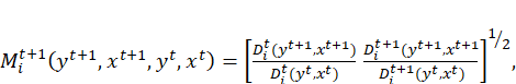(2)

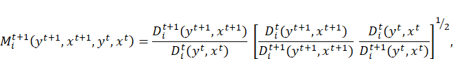
The index is defined as the geometric mean of two MPIs. Caves et al. (1982) assume that ( and ( are equal unity for each observation and period, which means that there is no technical efficiency (Farrel, 1957). When >1, productivity increases; when <1, there is a reduction in productivity performance; and =1 signifies no change in productivity from periods t to t+1. Färe et al. (1994) follow the assumptions of Farrel (1957) that technology is linear and allows for inefficiencies. These assumptions allow the productivity index to be decomposed into two components: efficiency change and technical change (change in the technological frontier). Thus, equation (2) can be written as follows:

(3)

where the quotient outside the bracket indicates the TEC and the shift in the frontier or TC between periods t and t+1 is represented by the ratios inside the bracket. From the equation, some characteristics may be noted: shifts in technology are measured for the observations at t and t+1; technology does not need to behave uniformly; and, lastly, there is the possibility of technological regress. In another notation, we can use the following statement:

TEC measures the change in relative efficiency or how close is the distance of observation to the frontier in period t+1 compared with period t. If TEC=1, then there is no change in efficiency in periods t+1 and t relative to the distance of the frontiers. If TEC>1, then the observation moved to period t+1 from its original position in period t, and if TEC<1, then the reverse condition occurred. Another effect is the change in technology (i.e., TC) between periods t and t+1. If TC=1, then there is no shift in the technological frontier; when TC>1, there is technological progress from periods t to t+1; and if TC<1, then there is technological regress (Färe et al., 1994).

Regarding the interpretation of the shifting effect on the frontiers, growth in production is obtained when the MPI (i.e., TFP) is above one (TFP > 1); vice versa, there is production regression when TFP < 1. The MPI sets the measurement of productivity movements using multi-input and multi-output data (Caves et al., 1982). As another feature, the model allows physical unit data, and no price index problem arises. This study follows the input-based MPI developed by Färe et al. (1994). The application of the MPI score components is further explained in the estimation results section, and the MPI scores are available in tables (4)-(7). The application of the MPI score components is further explained in the estimation results section.

3.3. The Relationship between Fiscal Decentralization and Government Expenditure Efficiency – Data and the Baseline Model

The main objective of this research is to measure the effect of the degree of fiscal decentralization on government expenditure efficiency. After measuring the MPI in the first step, the second step in the two-step procedure consists of analyzing the effect of the degree of fiscal decentralization on government expenditure efficiency using a Tobit model. The baseline model to correspond with a censored model similar to that in this study takes a general form as follows:

(4)

where  denotes the MPIs of the four types of expenditures, i.e., infrastructure, education, health and social protection, obtained from the first step in this study;  is the time effects common to all provinces in the sample;  is the focal explanatory variables and the control variables in the model. The subscripts i and t denote time and province, and  is the error term. The predicted values must be lower than unity to be censored, as the requirement to regress the Tobit model. Our data sample consists of 26 provinces in the 2004-2015 period (similar to the data sample included in the measurement of the MPI), and a panel data Tobit model with bootstrapped standard errors is utilized to deal with a censored regression estimation. The estimation results are presented in table (8) for each type of expenditure.

The dependent variable (gee) employs the MPIs for infrastructure, education, health and social protection expenditures. We construct two measures of fiscal decentralization as the main explanatory variables. The first is the total expenditure of a regional government as a share of the total expenditure of the central government and the corresponding regional government, and the second is the total tax revenue of a regional government as a share of the total tax revenue of the central government and the corresponding regional government. Some scholars, such as Stegarescu (2005), Fiva (2006), and Adam et al. (2014), have adopted similar measures. Expenditure decentralization (expdec) corresponds with the size of the regional government size in relation to the central government. Moreover, tax revenue decentralization (taxdex) is constructed from the local tax revenue collected by the regional government, and it is different from the tax revenue given or shared by the central government. Tax revenue decentralization represents a region’s ability to finance its expenditures without the contribution of the central government. Higher values of the two variables reflect higher levels of decentralization.

Several control variables that affect government expenditure efficiency are included in the estimation. All data for the control variables are obtained from Statistics Indonesia. The first variable controls for the level of productivity and the scale of the economy, and we use the real regional gross domestic product per capita (ecscale). From a theoretical perspective, a wealthier province, as shown by a higher GDP per capita, is expected to have greater productivity than a province that is not wealthy, and this greater productivity increases the region’s government expenditure efficiency. Population density (popdensity) represents the level of jurisdiction of a regional government. The variable represents both the service area controlled by the regional government and the size of the population. Population density is measured by the number of people per square km. Another variable is total population (totalpop), which controls for economies of scale.

Two socioeconomic measures are introduced: first, the ethnolinguistic fractionalization index (ethno) and, second, the political stability index (politics). Ethnolinguistic fractionalization is defined as a measure of the probability that two randomly selected individuals are not from the same ethnolinguistic group (Hudson and Taylor, 1972), and this index ranges from 0 to 1, with a higher value indicating a higher level of heterogeneity. The variable is obtained from Arifin, Evi Nurvidya et al. (2015) and is available for provinces in Indonesia. The political stability index ranges between 0 and 100, and a higher value represents a more stable political condition. The descriptive statistics and simple correlation matrix are presented in tables (2) and (3). From table (3), the correlation coefficients of the main explanatory variables are below 0.8, indicating that there is no severe multicollinearity problem in the data set.

Table 2. Descriptive Statistics – Tobit

Table 3. Simple Correlation – Tobit

4. Estimation Results and Discussion

4.1. Government Expenditure Efficiency – The Malmquist Productivity Index

The MPI model allows productivity to be defined by several inputs and outputs, and productivity is measured as the ratio of the index of the level of the inputs and outputs and a change in this ratio between times t and t+1, which reflects a change in the productivity of government expenditure. The model considers the fact that during the period of the data sample, the productivity of governments can improve or deteriorate, showing a shift in the frontier because of the TC that has been applied by the government. In this study, an input-oriented MPI is estimated, and the TPF index (TFPC) can be broken down into TEC and TC. The TEC index captures the diffusion effect or performance that is catching up, such as an improvement in several aspects such as (1) institutional quality, (2) management, (3) investment, (4) planning, and (5) budgeting. The TC index represents an upgrading innovation or a shifting along the frontiers due to technological improvement.

The analysis will be discussed as follows. First, the overall performance of the TFP of each type of expenditure is examined using the mean of the TFP indices of all provinces within the sample period. Second, the performance of the TEC and TC of the provinces within the sample period is assessed by evaluating the mean of the TEC and TC of all provinces. There are some possible explanations, but we limit the discussion to four combinations. The evaluation is based on the TFPC, TC and TEC indices. If the indices are larger than 1, then there is upgrading or improvement in technical efficiency or technology, whereas if the indices are smaller than 1, then government expenditure performance seems to face technical inefficiency or technological deterioration. In the first combination, the TC and TEC indices are greater than 1, showing that both changes improve significantly over the years. In the second combination, the TEC index is greater than 1, while the TC index is lower than 1. In the third combination, the TEC index is lower than 1, while the TC index is greater than 1. Lastly, in the fourth combination, both the TEC and TC indices are lower than 1. The MPI results are presented in tables (4), (5), (6), and (7) for infrastructure, education, health and social protection, respectively.

Table 4. Infrastructure MPI

Note: There is a slight difference in the calculation of the average values because the results are rounded to two decimal points.

Table 5. Education MPI

Note: There is a slight difference in the calculation of the average values because the results are rounded to two decimal points.

Starting with infrastructure expenditure, table (5) shows that the mean of the TFPC index is lower than 1, i.e., 0.86. The total productivity of infrastructure expenditure for all regional governments over the 12-year period cannot achieve a significant improvement. For the 26 provinces, we can rank their TFPC indices and conclude that North Sumatra, DI Yogyakarta and Nanggroe Aceh Darussalam are the provinces with the highest TFPC indices.

In contrast, West Sumatra, Southeast Sulawesi and Central Sulawesi are the three provinces with the lowest productivity. Regarding TEC and TC performance, no provinces have both TEC and TC indices larger than 1. Interestingly, most provinces, excluding North Sulawesi, Bengkulu and West Kalimantan, are found to have upgrading performance in technical efficiency, as represented by TEC indices larger than 1; North Sulawesi, Bengkulu and West Kalimantan have TEC indices smaller than 1. Moreover, all provinces fail to gain an improvement in TC, as indicated by TC indices smaller than 1.

The MPI results for education expenditure are presented in table (6). From the findings, the mean MPI for education reveals a high score larger than 1, i.e., 1.15. The index suggests that the overall productivity of government in the education sector improves significantly within the sample period for all provinces. All provinces show an upgrading in TC, as shown by TC scores larger than 1. Most provinces demonstrate an increase in performance with regard to both TEC and TC, as shown by TEC and TC scores larger than 1; however, West Kalimantan, North Sulawesi, Bengkulu have TEC indices lower than 1, which indicate their lower efficiency in providing public services in the education sector.

Table 6. Health MPI

Note: There is a slight difference in the calculation of the average values because the results are rounded to two decimal points.

Table 7. Social Protection MPI

Table 4. Infrastructure MPI

Note: There is a slight difference in the calculation of the average values because the results are rounded to two decimal points.

Table 5. Education MPI

Note: There is a slight difference in the calculation of the average values because the results are rounded to two decimal points.

Starting with infrastructure expenditure, table (5) shows that the mean of the TFPC index is lower than 1, i.e., 0.86. The total productivity of infrastructure expenditure for all regional governments over the 12-year period cannot achieve a significant improvement. For the 26 provinces, we can rank their TFPC indices and conclude that North Sumatra, DI Yogyakarta and Nanggroe Aceh Darussalam are the provinces with the highest TFPC indices.

In contrast, West Sumatra, Southeast Sulawesi and Central Sulawesi are the three provinces with the lowest productivity. Regarding TEC and TC performance, no provinces have both TEC and TC indices larger than 1. Interestingly, most provinces, excluding North Sulawesi, Bengkulu and West Kalimantan, are found to have upgrading performance in technical efficiency, as represented by TEC indices larger than 1; North Sulawesi, Bengkulu and West Kalimantan have TEC indices smaller than 1. Moreover, all provinces fail to gain an improvement in TC, as indicated by TC indices smaller than 1.

The MPI results for education expenditure are presented in table (6). From the findings, the mean MPI for education reveals a high score larger than 1, i.e., 1.15. The index suggests that the overall productivity of government in the education sector improves significantly within the sample period for all provinces. All provinces show an upgrading in TC, as shown by TC scores larger than 1. Most provinces demonstrate an increase in performance with regard to both TEC and TC, as shown by TEC and TC scores larger than 1; however, West Kalimantan, North Sulawesi, Bengkulu have TEC indices lower than 1, which indicate their lower efficiency in providing public services in the education sector.

Table 6. Health MPI

Note: There is a slight difference in the calculation of the average values because the results are rounded to two decimal points.

Table 7. Social Protection MPI

In table (7), the health productivity indices can be evaluated. The overall mean TFPC over the 12-year period for all provinces reveals a score lower than one. We rank the provinces with the highest TFPC scores, and North Sumatra, Jambi and DI Yogyakarta perform as the top three provinces. In contrast, the provinces with the three lowest mean TFPC scores are Nanggroe Aceh Darussalam, Bengkulu and Bali. The main reason for these low TFPC scores is that all provinces fail to improve their technology in the health sector, while most provinces manage to perform better in increasing their efficiency performance. Only West Kalimantan, Nanggroe Aceh Darussalam and Bali are struggling to boost their efficiency performance.

Focusing on social protection expenditure, West Sumatra, North Sumatra, Jambi, East Nusa Tenggara, Lampung, Central Kalimantan and West Java are able to advance their productivity, as shown by a mean TFPC score higher than one, while 19 provinces scored lower than one. The overall mean TFPC score for all provinces reveals the downgrading productivity of the government in delivering social protection services. From the TC evaluation, all provinces tend to fail to increase their performance, as demonstrated by TC scores lower than one. In contrast, most provinces succeed in improving their TEC performance, except for six provinces (South Sumatra, West Nusa Tenggara, DI Yogyakarta, North Sulawesi and Nanggroe Aceh Darussalam).

The discussion of the MPI scores may bring more insights than the rest of our discussion in this paper, particularly in regard to policy recommendations. Regional governments can use the MPI scores to evaluate their performance in relation to other provinces. Bali has a lower mean TFPC score for infrastructure, health and social protection expenditures. The TC indices for these three types of expenditures remain lower than one. One possible explanation is that Bali is a province with tourism as the main contributing sector; it is likely that the government places more emphasis on developing the tourism sector. There is room for the performance of Bali to catch up with the performance of other provinces by improving its innovation in the infrastructure, health and social protection sectors. In contrast, North Sumatra manages to increase its productivity performance in three sectors: education, health and social protection; additionally, it demonstrates a mean TFPC score higher than one. Although its mean TFPC score in infrastructure reveals a lower score, North Sumatra succeeds in promoting technical efficiency in infrastructure. Another benefit of the analysis using the MPI model is that we are able to assess the performance of a province during the period.

From the above discussion, MPI scores can be used to evaluate government productivity performance. As another application, the indices can be employed in the regression to capture the relationship between the degree of fiscal decentralization and government expenditure efficiency. The yearly TFP values for the four types of expenditures are utilized as the dependent variable in the subsequent empirical analysis using the Tobit model.

4.2 Fiscal Decentralization and Government Expenditure Efficiency

Before discussing the findings from the estimation, it is important to begin with the model specifications in table (8). The dependent variable in table (8) is the TFPC scores for infrastructure, education, health, and social protection expenditures. Regarding the explanatory variables in columns (1) and (2), expenditure decentralization is assessed using three other control variables: the economic scale, population density and total population. The effects of ethnolinguistic fractionalization and political stability on government expenditure efficiency are introduced in column (2). Moreover, the impact of tax revenue decentralization is emphasized separately in columns (3) and (4), including the economic scale, population density and total population. The ethnolinguistic fractionalization index and politic stability are included in the estimation in column (4) to assess the institutional effect on government efficiency.

From the estimation results in table (8), expenditure decentralization promotes infrastructure efficiency and is statistically significant in column (1). The size of the economic scale is found to be an efficiency-enhancing factor in all estimations. Population density appears to positively affect government efficiency in the infrastructure sector in all estimations. The size of the total population indicates that it stimulates government efficiency. Ethnolinguistic fractionalization positively contributes to enhancing the efficiency index for infrastructure. Political stability is proven to promote the government infrastructure efficiency index.

The inclusion of nondiscretionary variables (ethno and politics) affects the magnitude of the decentralization variables in columns (2) and (4), and they become statistically nonsignificant, while the effect on government efficiency remains positive. In addition, the degree of decentralization using tax revenue obtained from the local contribution is found to have a positive effect on efficiency in column (3) and becomes statistically nonsignificant after introducing the ethnolinguistic fractionalization index and the political stability index in column (4). Both decentralization measurements confirm the hypothesis that given a higher degree of fiscal decentralization, local governments tend to improve their performance and work more efficiently. The estimation results for education expenditure efficiency indicate that expenditure and the degree of tax revenue decentralization positively affect government efficiency in columns (1) and (3), with the effect being statistically significant at the 1 percent level; however, the magnitude of the degree of tax decentralization appears to be the cause of a decrease in government efficiency when controlling for the institutional variables. In line with infrastructure and education expenditures, the degree of fiscal decentralization, particularly in health expenditure, promotes government efficiency in columns (1)-(3). In contrast, an increase in the degree of tax decentralization seems to create more inefficiency in the social protection sector in column (4) after controlling for the institutional variables. The overall estimation results agree with the findings of Arsana (2014) but are the opposite of the findings of Tirtosuharto (2019). Possible reasons for the different estimation results are the differences in the methodologies used to measure efficiency, the input and output data and the sample period.

Table 8. Effect of Fiscal Decentralization on Government Expenditure Efficiency – Tobit Model

Note: The dependent variables are infrastructure, education, health and social protection Malmquist productivity indices (TFPC) from the first stage computation. The asterisks represent the p-value significance levels (*p<0.1; **p<0.05; ***P<0.01). Standard errors are in parentheses.

5. Conclusion

Notably, this study on government expenditure efficiency evaluates government performance in four important sectors, i.e., infrastructure, education, health and social protection, after the implementation of fiscal decentralization in Indonesia. Using an MPI approach, the results reveal that local governments have managed to improve their efficiency in these four types of expenditures. The TEC and TC in infrastructure, health and social protection tend to deteriorate over the years; in contrast, education expenditure succeeds in maintaining higher efficiency. An important aspect of this study is that it assesses the effect of the degree of fiscal decentralization on government efficiency. The estimation results confirm that the implementation of fiscal decentralization encourages local government to work efficiently and to use budget resources for appropriate development projects in accountable and transparent ways.

Despite the lack of data available at the provincial level to measure the output of government performance, the MPI is highly conducive to measuring the productivity and efficiency of regional governments in Indonesia. Our empirical findings may significantly contribute to policy evaluations and act as an instrument to evaluate government performance.

References

1. Adam, A., Delis, M. D. and Kammas, P., 2014. Fiscal decentralization and Public Sector Efficiency: Evidence from OECD Countries. Econ Gov, 15, pp.17-49.
2. Afonso, A., Schuknecht, L. and Tanzi, V., 2005. Public Sector Efficiency: an International Comparison. Public Choice, 123, pp.321–347.
3. Afonso, A. and Fernandes, S., 2006. Measuring Local Government Spending Efficiency: Evidence for the Lisbon Region. Regional Studies, 40, pp. 39–53.
4. Afonso, A., Schuknecht, L. and Tanzi, V., 2006. Public Sector Efficiency: Evidence for the New EU Member States and Emerging Markets. Working Paper no. 581. Frankfurt: European Central Bank.
5. Afonso, A., Schuknecht, L. and Tanzi, V., 2010. Public Sector Efficiency: Evidence for New EU Member States and Emerging Markets. Applied Economics, 42, pp. 2147-2164.
6. Afonso, A. and St. Aubyn, M., 2005. Non-parametric Approaches to Public Education and Health Efficiency in OECD Countries. Journal of Applied Economics, 8, pp.227–246.
7. Afonso, A. and St. Aubyn, M., 2006. Cross-country Efficiency of Secondary Education Provision: a Semi-parametric Analysis with Non-discretionary Inputs. Economic Modelling, 23, pp. 476–491.
8. Alesina, A. and La Ferrara, E., 2005. Preferences for Redistribution in the Land of Opportunities. J Public Econ, 89, pp.897–931.
9. Arifin, E. N., Ananto, A., Utami, D. R. W., Handayani, N. B. and Pramono, A., 2015. Quantifying Indonesia's Ethnic Diversity. Asian Population Studies, 11, pp. 233-256.
10. Besley, T. and Case, A. 1995. Incumbent Behavior: Vote-seeking, Tax-setting, and Yardsick Competition. Am Econ Rev, 85, pp., 25–45.
11. Besley, T. and Smart, M., 2007. Fiscal Restraints and Voter Welfare. J Public Econ, 91, pp.755–773.
12. Caves, D. W., Christensen, L. R. and Diewert, W. E. 1982. The Economic Theory of Index Numbers and the Measurement of Input, Output, and Productivity. Econometrica, 50, pp. 1393-414.
13. Clements, B., 2002. How Efficient is Education Spending in Europe? European Review of Economics and Finance, 1, pp. 3–26.
14. Enikolopov, R. and Zhuravskaya, E., 2007. Decentralization and Political Institutions. J Public Econ, 91, pp.2261– 2290.
15. Fa¨re, R., Grosskopf, S. and Lovell, C. A. K. 1994. Production Frontiers. Cambridge: Cambridge University Press.
16. Farrell, M. 1957. The Measurement of Productive Efficiency. Journal of the Royal Statistical Society Series A (General), 120, pp. 253–281.
17. Fiva, J., 2006. New Evidence on the Effects of Fscal Decentralization on the Size and the Composition of Government Spending. FinanzArchiv, 62, pp.250–280.
18. Fisman, R. and Gatti, R., 2002. Decentralization and Corruption: Evidence Across Countries. J Public Econ, 83, pp. 325–346.
19. Hindriks, J. and Lockwood, B., 2009. Decentralization and Electoral Accountability: Incentives, Separation, and Voter Welfare. Eur J Polit Econ, 25, pp.385–397.
20. Hudson, M. C. and Taylor, C. L. 1972. World Handbook of Political and Social Indicators. Yale University Press.
21. Mihaiu, D. M., Opreana, A. and Cristescu, M. P., 2010. Efficiency, Effectiveness and Performance of the Public Sector. Romanian Journal of Economic Forecasting, 4, pp. 132-147.
22. Myerson, R., 2006. Federalism and Incentives for Success of Democracy. Q J Polit Sci, 1, pp.3–23.
23. Nishimizu, M. and Page, J. M. 1982. Total Factor Productivity Growth, Technological Progress and Technical Efficiency Change: Dimensions of Productivity Change in Yugoslavia, 1965-78. The Economic Journal, 92, pp. 920-36.
24. Tirtosuharto, D., 2010. The Impact of Fiscal Decentralization and State Allocative Efficiency on Regional Growth in Indonesia. Journal of International Commerce, Economics and Policy, 1, pp. 287-307.
25. Prud’homme, R. 1995. On the Dangers of Decentralization. World Bank Res Obs, 10, pp.201–220.
26. Stegarescu, D., 2005. Public Sector Decentralization: Measurement Concepts and Recent International Trends. Fiscal Stud, 26, pp.301–333.

Article Rights and License

Corresponding Author