Evaluation of Options using the Black-Scholes Methodology

KeywordsBlack-Scholes equation Monte Carlo simulation stochastic

JEL Classification B41, C02, G13

Full Article

1. Introduction

This paper presents the Black-Scholes methodology and the application of this methodology on the underlying asset of the nature of the listed stock on the Bucharest Stock Exchange (Bvb.ro, 2018a). The results obtained are then compared to our results in an article where we determined the values for Call and Put by Monte Carlo simulation.

The Black-Scholes equation was developed in 1969 by Fisher Black and Myron Scholes, but was published in 1973 with the appearance in Chicago of the first regulated market of negotiable options. The mathematical model developed by Fisher Black and Myron Scholes for the evaluation of derivative products of the nature of the options was subsequently developed by Robert Merton. It is noteworthy that for this scientific contribution, Myron Scholes and Robert C. Merton receive the Nobel Prize for Economics in 1997 (the Swedish Academy of Sciences highlights the contribution of Fisher Black who was no longer alive at the time of the award).

The Black-Scholes mathematical model offers investors a rational way to evaluate options and is seen as a very important contribution to finance (Copeland and Weston, 1988, p.276).

According to some authors (Taleb, 2008, p. 314), Black, Scholes and Merton have only improved an old mathematical formula. "It had a long list of precursors forgotten, including the mathematician and player Ed. Thorp who wrote the successful book „Bet on the croupier”, but people came to think that it was invented by Scholes and Merton, though in fact they did it acceptable." However, the mathematical model is one accepted by academia and industry, but it is also criticized because it integrates the normal distribution (gaussian distribution), which does not take into account that markets are characterized by extreme events. The normal distribution is based on the idea that most observations refer to the average and as a result, the probability of a deviation from the mean drops exponentially as you move away from the average (Taleb, 2008, p. 265).

What we can see is that if the extreme events on financial markets are excluded, the equation gives a reasonable price of derivative products of the nature of the options, it provides coverage of the investment risk, but if reality does not confirm this, then things become extremely difficult for those who they hold such financial instruments and for society as a whole. This was evident in the financial crises of 1998 (the Russian financial crisis) and the one in 2017. But the financial sector, with the Black-Scholes equation, has developed a set of associated equations for various assumptions for the various financial instruments, losing sight of that the equation is based on the very low probability of extreme events. In the equation, the underlying asset follows a random walk on a continuous time, meaning it obeys the Brownian motion model and the consequence of the Brownian motion model of Bachelier is that fluctuations in the stock markets are very rare and practical it should never occur (Stewart, 2013, p. 265). A process is called random walk if the particle receives random impulses and the direction of each impulse is subject to the normal distribution law, and the Brownian motion is a continuous-time version of such random walks.

2. Literature Review

The first article that empirically examines the Black-Scholes model is written by MacBeth and Merville (1979). More recently, empirical studies are found in Sarkar (1995) and Çetin et al (2006). An empirical examination of the Black-Scholes model is carried out by McKenzie, Gerace and Subedar (2007). About the robustness of the model we find an article well-structured by Karoui, Picqué and Shreve (1998). Extensions of the model in the form of jump diffusion are found in Merton (1976) and more recently in Kou (2002). A critique of the Black-Scholes model can be found at Haug and Taleb (2011). This being said, a review of recent developments in the Black-Scholes models is synthesized by Saedi and Tularam (2018).

3. Methodology

3.1. Black-Scholes Equation

The hypotheses of the Black-Scholes theory are (Black and Scholes, 1973, p. 740):

„the short-term interest rate is known and is constant through time; the stock price follows a random walk in continuous time with a variance rate proportional to the square of the stock price. Thus, the distribution of possible stock prices at the end of any finite interval is lognormal. The variance rate of the return on the stock is constant; the stock pays no dividends or other distributions; the option is "European," that is, it can only be exercised at maturity; there are no transaction costs in buying or selling the stock or the option; it is possible to borrow any fraction of the price of a security to buy it or to hold it, at the short-term interest rate; there are no penalties to short selling. A seller who does not own a security will simply accept the price of the security from a buyer, and will agree to settle with the buyer on some future date by paying him an amount equal to the price of the security on that date”.

Given the above assumptions, we consider a function V = V(S,t) representing the value of the option and note with  the value of the portfolio consists of a long position on a derivative unit and a short position on a  quantity of the underlying asset. On the basis of these notations we can write successively the following (see Wilmott, 2007, pp. 141-143):

The value of the portfolio consisting of a long position on a derivative unit V and a short position on a quantity, denoted , of the underlying assetS, is given by the following expression:

(1)

The underlying asset price has the following dynamic equation:

(2)

The dynamics of the portfolio value from t to t+dt is given by the following expression:

(3)

If V=V(S,t), using Taylor serial development, we will get:

(4)

Where:

(5)

From (4) and (5), by substitution, we obtain:

(6)

From (3) and (6), by substitution, there is obtained:

(7)

Portfolio risk is given by the terms that contain dS, respectively  and . To eliminate portfolio risk, these terms of the equation must be zero, ie . What we notice is that if we choose  then the portfolio risk is zero and as a result, the equation of movement of the value of the portfolio is completely risk-free and has the following expression:

⇒ (8)

If the change in the value of the portfolio is completely risk-free, then this is equivalent to depositing a sum of money, the size of the portfolio value, into a bank account, remunerated at a risk-free interest rate (r). As a result, we can write the following expression:

(9)

By equalizing the expressions in equations (8) and (9) we obtain:

(10)

From equation (1) we know the value of the portfolio . Knowing that  , then . Under these conditions, by substituting  in equation (10) there is obtained:

(11)

This last expression - equation (11) - is the Black-Scholes equation.

3.2. Explicit Solutions for Call and Put

Black - Scholes equation does not tell us which option category (Call or Put) is valued and the exercise price or maturity. The value of an option is a function of the underlying asset at the maturity date (t=T). This means that a function V(S_T,T) representing the profit or loss at maturity should be written. So, if we have a Call option then we know that [Wilmott, 2002, p. 97]:

V(,T) = max(S_T -E, 0) = Payoff (S) (12)

Under a neutral risk probability (Q), the option price is given by the expectation of payoff (E^Q) updated at the risk-free interest rate as follows:

C = V(S,t) = (13)

The mathematical expectation of a random variable X of the continuous type is given by the following expression (Bratian et al, 2016, p. 222):

(14)

Applying the expression (14) in the expression (13), we have:

C = (15)

⇒

(16)

The price of the underlying asset at maturity (S_T) can be written as follows: , where R =  represents the profitability of the underlying at maturity. Therefore, S_T = S, and C can be rewritten:

(17)

Whereas R is subject to normal law, the distribution density of R, f(R) is given by the following expression:

(18)

By substituting in expression (17) the expression (18) we obtain:

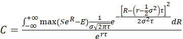(19)

The above expression can thus be written:

(20)

To remove the "max" function from the expression (20), we use that  and consequently (Negrea, 2006, p. 138):

(21)

Having said this, after changing the variables in the integers of equation (21) and taking into account the symmetry property of the normal distribution law, we will obtain the explicit solution for Call:

(22)

where: ;

Next, the explicit solution for the Put option can be determined quite easily, knowing the explicit solution for Call.

The Call-Put parity theorem tells us that:

(23)

By replacing the relation (22) in equation (23), we will have:

(24)

4. Evaluation of Options with Underlying Asset of Compa SA Shares Using the Black-Scholes Methodology

Next, we will apply the methodology described above on underlying asset of the type of stock that does not pay a dividend. We consider the underlying asset to be Compa SA's (Bvb.ro, 2018b) shares. The time series used to calculate the volatility of the underlying asset is between 19 July 2017 and 10 August 2018 and the risk-free interest rate is 3.31% (Bnr.ro, 2018). In the analysis, the price of the underlying asset is considered to be the closing price. The strike price is considered at the money . We consider maturities at 3 months (τ = 0.25), 6 months (τ = 0.5), 9 months (τ = 0.75) and 1 year (τ = 1) from 10 August 2018.

As a result:

- for the 3-month maturity, we have:

=

 =

- for the 6-month maturity, we have:

=

 =

- for the 9-month maturity, we have:

=

 =

- for the 12-month maturity, we have:

=

 =

5. Conclusions

Following calculations, we can state the following (see Table 1):

Table 1. Call / Put value

Source: own calculations

References

1. Black, F. and Scholes, M., 1973. The Pricing of Options and Corporate Liabilities. The Journal of Political Economy, 81(3), pp. 637-654.
2. BNR, 2018. Emisiune pe piata primara [online] Available at: http://www.bnr.ro/Emisiuni-pe-piata-primara5651.aspx [Accessed on 11 September 2018].
3. Brătian, V., 2018. Evaluation of Options using the Monte Carlo Method and the Entropy of Information. Expert Journal of Economics, 6(2), pp. 35-43.
4. Brătian. V. (coordinator), Bucur, A. and Opreana, C., 2016. Finanțe cantitative – Evaluarea valorilor mobiliare și gestiunea portofoliului. Editura ULBS, Sibiu.
5. BVB.ro, 2018a. Bucharest Stock Exchange [online] Available at: www.bvb.ro [Accessed on 11 September 2018].
6. BVB.ro, 2018b. Financial Instruments – Compa SA [online] Available at: http://www.bvb.ro/FinancialInstruments/Details/FinancialInstrumentsDetails.aspx?s=CMP [Accessed on 11 September 2018].
7.  Çetin, U., Jarrow, R., Protter, P. and Warachka, M., 2006. Pricing Options in an Extended Black Scholes Economy with Illiquidity: Theory and Empirical Evidence. The Review of Financial Studies, 19(2), pp. 493-529.
8. Copeland, Th., Weston, F., 1988. Financial Theory and Corporate Policy, 3^rd edition. Boston, USA: Addison-Wesley Publishing.
9. Haug, E. and Taleb, N., 2011. Option treders (very) sophisticated heuristics, never the Black-Scholes-Merton formula. Journal Behavior & Organization, 77, pp. 97-106.
10. Karoui, N., Jeanblanc- Picqué, M. and Shreve, S., 1998. Robustness of the Black and Scholes formula. Mathematical Finance, 8(2), pp. 93-126.
11. Kou, S.G., 2002. A Jump-Diffusion Model for Option Pricing. Management Science, 48(8), pp. 1086-1101.
12. MacBeth, J. and Merville, L., 1979. An Empirical Examination of the Black-Scholes Call Option Pricing Models. The Journal of Finance, 34(5), pp. 1173-1186.
13. McKenzie, S., Gerace, D. and Subedar, Z., 2007. An empirical investigation of the Black-Scholes model: evidence from the Australian Stock Exchange. Australasian Accounting, Business and Finance Journal, 1(4), pp. 71-82.
14. Merton, R., 1976. Option Pricing When Underlying Stock Returns Are Discontinuous. Journal of Financial Economics, 3, pp. 125-144.
15. Negrea, B. and Damian, V., 2015. Calcul stochastic aplicat în ingineria financiară. București: Editura Economică.
16. Negrea, B., 2006. Evaluarea activelor financiare – o introducere în teoria proceselor stocastice aplicate în finanțe. București: Editura Economică.
17. Saedi, Y. and Tularam, G., 2018, A Review of the Recent Advances Made in the Black-Scholes Models and Respective Solutions Methods. Journal of Mathematics and Statistics, 14(1), pp. 29-39.
18. Sarkar, S., 1995. Black-Scholes, As Compared to Observed Price: An Empirical Study. Managerial Finance, 21(10), pp. 1-8.
19. Stewart, I., 2013. 17 Ecuații care au schimbat lumea. București: Editura Paralela 42.
20. Taleb, N., 2008. Lebăda Neagră. București: Editura Curtea Veche.
21. Wilmott, P., 2002. Derivative. Inginerie financiară. Teorie & practică. București: Editura Economică.
22. Wilmott, P., 2007. Introduces Quantitative Finance. Chichester, England: John Wiley & Sons.

Article Rights and License

Corresponding Author