KeywordsCOVID-19 Laplace distribution nonlinear regression Taiwan stock index futures (TF) Taiwan stock price index (TAIEX)
JEL Classification HC51, C52, G13
Full Article
1. Introduction
This paper intends to discuss the changes for dependence tendencies (or called the associations) for the return rates of stock price indices and stock index futures before and during coronavirus (COVID-19) pandemic periods. The futures is a kind of financial derivatives and a hedging instrument (Hull, 2003; Johnson, 1980; Junkus et al., 1985; Park and Switzer, 1995). COVID-19 is a terrible disaster around the world till now and hit the economic, public health, and social living statuses. In particular, the stock price indices of the investing during COVID-19 climb higher than those before COVID-19. Thus, it would be interesting to discuss the associations between the stock price index and stock index futures. This is because the latter has the function of price discovery, which relates to the current stock price index.
Although the discussions of literature on the futures are always from the views of time-varying dynamics (Mehlitz and Auer, 2021), price discovery (Chen et al, 2021; Yang et al, 2021), arbitrage trading, term structure (Fonseca and Gottschalk, 2013; Tan et al., 2021; Yang and Chen, 2021), this paper tries to analyze the Taiwan stock index futures (TF) that is a financial derivatives of Taiwan stock price index (TAIEX) regressed by the stock price index and the MSCI Taiwan index (MSCI_TWI), then intends to find what are the changes of associations among them before and during COVID-19. However, the regression analysis shall follow the assumptions such as Normal distribution and the linear model form. Almost analysis methods are based on the Normal distribution assumption, but the actual data cannot satisfy this assumption unless the researchers transfer the data using variable transformation or some other function transformation. To solve the problem of the Normal distribution assumption, Golden et al. (2019) mentioned that the researchers should try their best to estimate the regression to decrease the mistaken effect from the model form. They tried to correct the MLE of the coefficient estimation from the aspect probability distribution. However, the probability distribution of data has different parameters. Due to mathematical deviation is difficult to obtain for the MLE estimator and to reveal the effects of characteristics from the probability distribution. On the other way, they can directly test the probability distribution of data.
Based on the background and literature, the past regression analysis and time series method, which depend on Normal distribution and linear form assumptions seem not to be a good analytic tool for financial data. Therefore, two important keys that we should do are (1) checking the probability distribution of data and (2) finding the estimated nonlinear functions of data as possible as we can.
First, observations, in reality, are not always from Normal distribution. If we always use a Normal distribution assumption that does not match the data source, wrong critical values will result in unavoidable and uncontrollable risks arising from the hypothesis and testing in regression analysis. This is why the theories cannot analyze the nonstationary state or very complex data.
To confirm whether the probability models of the three kinds of return rates are from Normal distribution, we follow Wang and Lee (2019) to test the probability distributions by improved goodness of fit where 45 distributions are in the database used for hypotheses and testing. In the literature on the volatility of financial commodity price returns, the researchers almost used a series of ARCH models based on the assumption of Normal distribution to analyze them. Even with the regression analysis of data, no data-driven characteristics are concerned in the researches. For Normal distribution, the moments are invariance, especially the skewness and kurtosis coefficients. However, numerous data cannot satisfy the perfect assumption of Normal distribution. Researchers passively need to consider that the high-order moments will be affected by the change of probability distribution parameters to add the high-order moments into the model for discussion (Chen, Li, and Wang, 2011; Jondeau et al., 2021; Zaremba and Nowak, 2015). Therefore, finding correct probability distribution from testing plays an initial role in this paper to conjecture the return rates of TF, MSCI_TWI, and TAIEX. The improved goodness of fit can determine whether the data are satisfied with the characteristics of the Normal distribution.
Second, although econometrics exists the nonlinear regression or polynomial regression, researchers did not have a high willingness to analyze data with these two regressions. Therefore, the complex time-series data should be used the complex function form to fit so as to achieve the aim of accurate estimation. The advantage of accurate estimation is that the misspecification of function form for the expected values will not fall into the residuals which play a core role in the testing for regression analysis, such as heteroscedasticity and serial correlation.
As to build the regression model for the three kinds of return rates, only linear regression model form is not suitable for this paper to find the association of the three kinds of return rates. Nonlinear regression should not be the forms such as log, exponential, quadratic, cubic, and so on. We need more function forms to use in the nonlinear regression, for instance, the inverse function, absolute value function, trigonometric function, and so on. The advantage of nonlinear regression is that we can build a data-driven estimator and the function forms can tell us more information about the associations between the explanatory variable and the dependent variable.
Consequently, this paper proposes the financial data that include the trends of the TAIEX, TF, and MSCI_TWI before and during COVID-19. We test whether the three sets of data conform to the Normal distribution assumption of regression analysis, and then try to find the influence of COVID-19 on the three sets of data through the estimation formulas of nonlinear regression.
This paper proceeds as follows: Section 2 presents the methodology including the descriptions of data source and the theoretical methods of improved goodness of fit and nonlinear regression. Section 3 then describes the empirical research results and investigates the nonlinear estimators before, during COVID-19, and the whole observation period. Section 4 states the conclusion.
2. Research Methodology
2.1. Data Source and Description
We choose the daily after-hour close prices of nearby-month TF from Taiwan Futures Exchange (TAIFEX), the daily closing prices of MSCI_TWI, and TAIEX. TF and MSCI_TWI are financial derivatives, which are derived from TAIEX that is the main stock price index in Taiwan. It employs the daily data of three kinds of closing prices over the period from July 18, 2019, to September 30, 2020, for a total of 296 observations, downloaded from the TEJ database. The reason for choosing the time period is that COVID-19 spread before and during the time so as to show the substantial impact on the Taiwan stock and futures markets.
Figure 1 illustrates the trends of daily closing prices of TF, MSCI_TWI, and TAIEX. TF had occurred relatively low closing price from March to April in 2020. MSCI_TWI had relatively low closing prices during from July to December in 2019 and from May to June in 2020.
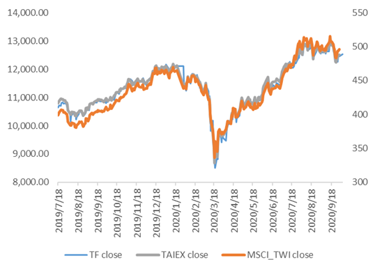
Figure 1. Trends of TX, MSCI_TWI, and TAIEX
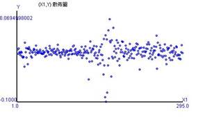
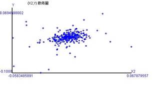
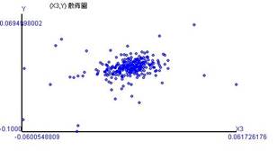
The daily return rate in this paper is calculated by the closing prices, with the formula as Rt = ln(Xi,t) – ln(Xi,t-1), as shown in Figure 2. The fluctuations of the daily return rates exhibit at the horizontal axis of the time variable, labeled by X1, in Figure 2-A. Figures 2-B and 2-C display the associations of the TF return rate(Y) and the MSCI_TWI return rates labeled by X2, and of that the TAIEX return rates labeled by X3.
Figure 2-A shows that the TF return rates in March of 2020 spread widely and can be divided into different degrees of deviation before and after COVID-19. The figure seems to have a horizontal correlation as a belt. Figures 2-B and 2-C show that the spots are concentrated in specific intervals, but there are still extremes.
The figures also show that the TF return rate has a positive linear correlation with the MSCI_TWI return rate (0.296) and with the TAIEX return rate (0.317), respectively. For instance, the correlation coefficient draws a linear association of 29.6% between the TF return rate and the MSCI_TWI return rate. We also can say that the TF return rate will increase by 29.6% when the MSCI_TWI return rate increases by 1%.
|
|
|
| (A) TF | (B) MSCI_TWI | (C) TAIEX |
Figure 2. Scatter plots of TX with time, MSCI_TWI and TAIEX
Table 1 summarizes the coefficients of descriptive statistics. The averages and the medians presenting the centralization tendency do not have consistent order results for the TF return rates and the TAIEX return rates. The averages show that MSCI_TWI return rate > TF return rate > TAIEX return rate. The medians show MSCI_TWI return rate > TAIEX return rate > TF return rate. The reason may be that the dispersion of return rates results in extremes affecting the representativeness of the averages. In addition, the averages and medians indicate negative skewness, implying that 295 observations cannot realize the property of Normal distribution. In particular, the kurtosis coefficients indicate the leptokurtic distributions of the three kinds of return rates, exceeding the kurtosis coefficient of Normal distribution. This finding is also in line with the dispersed extreme values shown in Figures 2-B and 2-C.
Table 1. Descriptive statistics
| variable |
|
|
|
|
| average | 148 | 0.000736 | 0.0005 | 0.000531 |
| median | 148 | 0.001619 | 0.001531 | 0.00107 |
| Standard deviation | 85.30338 | 0.013358 | 0.012334 | 0.016063 |
| Kurtosis coefficient | 1.8 | 8.079043 | 9.607588 | 15.04802 |
| Skewedness coefficient | 0 | -0.34964 | -0.74442 | -1.75073 |
| range | 294 | 0.126228 | 0.121781 | 0.169583 |
| minimum | 1 | -0.05835 | -0.06005 | -0.10008 |
| maximum | 295 | 0.06788 | 0.061726 | 0.0695 |
| coefficient of variation | 0.576374 | 18.15205 | 24.66936 | 30.23229 |
Note: X1,t is a time variable, X2,t is MSCI_TWI return rate, X3,t is TAIEX return rate, and Y is TF return rate
In the tendency of dispersion, the TF return rate has a risk of significant price changes, regardless of the standard deviations, ranges, or coefficients of variation. The standard deviations and the ranges reveal that TF return rate > MSCI_TWI return rate > TAIEX return rate. The coefficients of variation show that TF return rate > TAIEX return rate > MSCI_TWI return rate. In sum, the tendencies of concentration and dispersion indicate that three kinds of return rates have a high probability of not matching the characteristics of Normal distribution.
2.2. Methodology of the Testing Probability Distribution
For the verification methodology of the probability distribution, this paper follows Wang and Lee (2019) to conduct “improved goodness of fit” on three kinds of return rates, respectively. Since a sect of return rates has its specific numerical regularity, the mathematical function can be constructed and formed as the probability distribution. The “improved goodness of fit” is a test method based on the goodness of fit (Pearson chi-square test) to objectively judge the probability distribution of the data and determine the probability distribution from which the daily return rates come. The method describes as follows:
First, the null hypothesis of the improved goodness of fit needs to simulate data of a specific probability distribution, from which 100,000,000 random samples are extracted to construct the relative frequency distribution with K mutually exclusive classifications. The function of this relative frequency distribution tends toward the true specific probability distribution. Then we can calculate Ej = npj0 in the Pearson chi-square test to represent the distribution under the null hypothesis, where n is the number of observations in total; pj0 is the probability value of jth classification under the null hypothesis, and ![]() , j = 1, 2, …, k. The actual observations can be calculated and labeled as Oj. Then the Chi-square statistic is
, j = 1, 2, …, k. The actual observations can be calculated and labeled as Oj. Then the Chi-square statistic is
|
(1) |
where the degree of freedom is v = k – 1 – the number of point estimates. At the significant level, α%, we reject the null hypothesis when ![]() occurs, implying that the data set does not significantly own the characteristic of Normal distribution.
occurs, implying that the data set does not significantly own the characteristic of Normal distribution.
During this procedure, we simultaneously test the distributions with the point estimates in the data set. The first step is to estimate the point estimates of a parameter of a specific distribution and collect them as a data set.
The second step is to choose the optimal parameter under the null hypothesis with the same distribution depending on the minimum Chi-square test statistic. Each point estimate in the data set will run the “improved goodness of fit” under the null hypothesis of a specific distribution. The third step is to choose the optimal distribution with the optimal parameter. As for the methods of point estimation, there are UMVUE, MLE, and MME, respectively.
The advantage of the “improved goodness of fit” in this paper is that it can test 45 kinds of probability distributions for TF, MSCI_TWI, and TAIEX daily return rates, respectively. The minimum statistic of the Chi-square test is used as the probability distribution of data. In addition, the residuals from regression models can also be used for detecting the probability distribution using the same methodology of “improved goodness of fit”, which can effectively grasp the data status and characteristics.
2.3. Methodology of Nonlinear Regression
Testing probability distribution only shows the characteristics of TF, MSCI_TWI, and TAIEX return rates. The regression analysis can display the associations of these three before and during COVID-19. The mathematical functions of estimators are assisting us to compare the differences before and during COVID-19 so as to know how COVID-19 hit the financial market in Taiwan. However, it is very difficult to satisfy the assumptions of regression analysis that we mentioned Normal distribution and linear model. Regression model, ![]() , can be separated by two parts: the explainable part (
, can be separated by two parts: the explainable part (![]() ) and the unexplainable part (
) and the unexplainable part (![]() ). If the model form is wrong, then the model will become as
). If the model form is wrong, then the model will become as ![]() , where
, where ![]() is the mistake of wrong model form, which still exists in the residuals as the sample size becomes large enough (Lee and Wang, 2021). The mistake induces that the residuals reduce their representativeness and have biases. In this paper, we follow Wang and Lee (2019) to build the nonlinear regression model in which there are 37 nonlinear function forms for each explanatory variable to be transferred. Suppose a generalized regression model is
is the mistake of wrong model form, which still exists in the residuals as the sample size becomes large enough (Lee and Wang, 2021). The mistake induces that the residuals reduce their representativeness and have biases. In this paper, we follow Wang and Lee (2019) to build the nonlinear regression model in which there are 37 nonlinear function forms for each explanatory variable to be transferred. Suppose a generalized regression model is
|
|
(2) |
|
|
(3) |
where ![]() follows the probability distribution of
follows the probability distribution of ![]() satisfying
satisfying ![]() and
and ![]() ,i = 1, 2, 3. Zi( • ) is the nonlinear function of
,i = 1, 2, 3. Zi( • ) is the nonlinear function of ![]() . The nonlinear property is due to the transformation of
. The nonlinear property is due to the transformation of ![]() which should be calculated by 37 function forms. Since the linear association between the dependent variable and each explanatory variable, we choose as the optimal nonlinear function form (Zi( • )) using the highest correlation coefficient, that is max{r(Zi( • ),
which should be calculated by 37 function forms. Since the linear association between the dependent variable and each explanatory variable, we choose as the optimal nonlinear function form (Zi( • )) using the highest correlation coefficient, that is max{r(Zi( • ), ![]() )}, where r is the symbol of correlation coefficient. The main meaning of (3) is that we find the highest linear correlation of the transformed explanatory variable with
)}, where r is the symbol of correlation coefficient. The main meaning of (3) is that we find the highest linear correlation of the transformed explanatory variable with ![]() first, then regress the
first, then regress the ![]() on the transformed explanatory variables to get the estimated values (
on the transformed explanatory variables to get the estimated values (![]() ).
).
3. Analysis and Results
3.1. Results of Finding Probability Distributions
Although Table 1 has shown no characteristics of Normal distribution for three kinds of return rates, we shall test the probability distribution to know the characteristics of return rates. We investigate TF, MSCI_TWI, and TAIEX return rates and summarize them in Table 2.
After the “improved goodness of fit” of 45 probability distributions, we find that the chi-square test statistic is 5.661017, the smallest one in 45 probability distribution tests under the null hypothesis of the Laplace distribution with λ = 120.037749 and μ = 0.001070. We cannot significantly reject the null hypothesis by P-value (= 0.462347), so the TF return rate during the research period follows the Laplace distribution. The MSCI_TWI return rate has chi-square test statistic (= 4.623729) and P-value (= 0.593039) under the null hypothesis of the Laplace distribution with λ = 104.286294 and μ = 0.001619, so we cannot significantly reject the null hypothesis. The TAIEX return rate has chi-square test statistic (= 5.844068) and P-value (= 0.441219) under the null hypothesis of the Laplace distribution with λ = 131.179627 and μ = 0.001531, thus we cannot significantly reject the null hypothesis.
Table 2. Probability distribution testing of three kinds of return rates
| TF return rate | MSCI_TWI return rate | TAIEX return rate | |
| distribution | Laplace | Laplace | Laplace |
| λ | 120.037749 | 104.286294 | 131.179627 |
| μ | 0.001070 | 0.001619 | 0.001531 |
| Chi-square | 5.661017 | 4.623729 | 5.844068 |
| P value | 0.462347 | 0.593039 | 0.441219 |
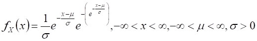
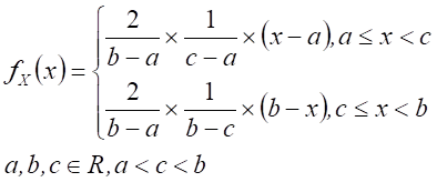
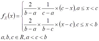
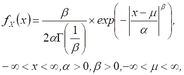
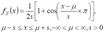
According to the above findings, the TF, MSCI_TWI, and TAIEX return rates follow the Laplace distribution whose probability density function is
|
|
(10) |
where ![]() is the probability density function form of the random variable, K, whose value is
is the probability density function form of the random variable, K, whose value is ![]() .
. ![]() is the shape parameter and
is the shape parameter and ![]() is the location parameter.
is the location parameter.
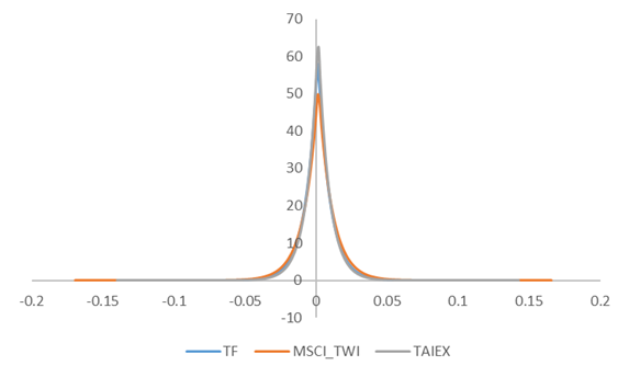
Figure 3. Probability distributions of TX, MSCI_TWI and TAIEX
The three kinds of return rates have their respective probability distributions under different parameters, as shown in Figure 3. The first feature is that the location parameter, μ, is the central point at the horizontal axis where the three values of μ are very close and around 0.00153. The shape parameter (λ) determines the height of the figure. The order of λ is TAIEX return rate (131.179627) > TF return rate (120.037749) > MSCI_TWI return rate (104.286294).
The second feature is that the Laplace distribution is a kind of leptokurtic distribution with long tails. The long tails indicate that it is possible to occur extreme returns with very low probability. This long-tail characteristic also arises in the shifted exponential distribution. In addition, the long tails of the MSCI_TWI return rate are longer than the other two, implying the possibility of occurrences for the very extreme return rates. The MSCI_TWI return rate has more distinct volatility than the other two.
The third feature is that the three kinds of return rates are not suitable to run the regression models under the assumption of Normal distribution, but are adaptable to run the analytic method in this paper considering the data-driven probability distribution. The fourth feature is that the Laplace distribution moves the shifted-exponential distribution by half to a negative value. If the random variable K follows the Laplace distribution, the absolute values of the random variable will follow the shifted exponential distribution with the parameter, 1 / λ.
Finally, the three kinds of return rates also have memoryless property that is a considerable property of the Laplace distribution and the shifted exponential distribution. This kind of property reveals that the market power dominates the market in economic and financial systems. For instance, under the condition of a previous return rate above 0.2%, the probability of the return rate above 0.3% (= 0.1% + 0.2%) will be the probability of the return rate above 0.1%.
3.2. Results of Nonlinear Regression before and during COVID-19
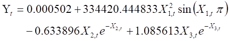
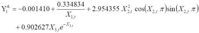
We run the nonlinear regression and obtain estimators (11), (12), and (13). (11) is the nonlinear estimator for the whole observation period and decomposes into the periodic trigonometric function of the time variable, the Xe-X function forms of the MSCI_TWI, and TAIEX return rates. Xe-X is a kind of convergent function toward zero as X approaches infinity.
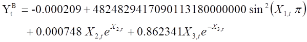
(12) and (13) are the estimator for the period before and during COVID-19, respectively. TF return rate in (12) is estimated and decomposed into the periodic trigonometric function of the time variable, the function of XeX for MSCI_TWI return rate, and the function of Xe-X for TAIEX return rate. TF return rate in (13) is estimated and decomposed into the inversed function of the time variable, the periodic trigonometric function for MSCI_TWI return rate, and the function of Xe-X for TAIEX return rate.
|
(11) |
|
(12) |
|
(13) |
3.2.1. Comparisons of the Effects for the Time Variable on TF Return Rate
The first main finding is the changes of the time variable functions. (12) of before COVID-19 and (11) of the whole observation period have the trigonometric function form of the time variable, but (13) is an inverse function of the time variable. At this point, we can compare the effect of each explanatory variable in (11) and (12) and find the difference between the data before considering the observation period and the data before COVID-19. The estimation of the TF return rates over the observation period is influenced by the period before and during COVID-19. Similar or identical functional forms occur in the time variable and the TAIEX return rate in (11). In other words, the data during the observation period and before COVID-19 dominates the dependence relationship of TF, MSCI_TWI and TAIEX.
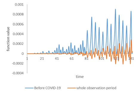
It is a surprising result that a time variable can display the periodic oscillation of the futures after the regression ran. Comparing the function value of each explanatory variable in (11) and (12) after nonlinear estimation, periodic oscillations occur in the functional form of time variables. We find that the time variable can capture the maturity characteristics of futures contracts. Figure 4-A demonstrates that the function of the time variable can show the characteristics of contract expiration for TF. The time variable function of (12) is the blue dot in the figure, showing that the rule is not obvious before the TF October contract (inclusive) of the 2019, and the periodic rule of 4~5 daily intervals occurs from November, 2019.
|
|
| (A) Before COVID-19 | (B) During COVID-19 |
Figure 4. The contributions of the time variable on the TF return rate
Second, we find that the time variable function dominated by the data before COVID-19 is a periodically trigonometric function in (11), but the fluctuation of the time variable function composed in (11) is obviously lower than (12) and the negative return rate is easy to occur. This is because (11) considers both the values of the variables over the observation period and the most appropriate dependency relationship coordinated by the four sets of variables (see (11) and the orange line in Figure 4-A).
The functions of the time variables during the observation period and before COVID-19 are up and down oscillation states. TF return rate before COVID-19 fluctuates more sharply over time and is all positive (see (12) and blue line in Figure 4-A). However, it is difficult to detect the regularity shown by the time variable function in (11). The nonlinear estimation results show that adding a time variable can show the characteristics of the futures contract expiration, and the functions of the time variable in (11) and (12) show that the fluctuation of the time variable function becomes more intense as the observation period is closer to COVID-19.
The trigonometric function form means that the time variable can grab the fluctuation of the TF return rates. The fluctuation with the time shows the characteristics of nearby month futures contracts having the settlement day and deliveries (see (11) and (12)). However, TF return rate cannot show the characteristics of the settlement day and deliveries using the time variable function during COVID-19 (see (13) and the blue line in Figure 4-B). We find that the time variable is invalid in grabbing the fluctuation of futures contracts because the increased time number after COVID-19 makes the TF return rates decrease.
3.2.2. The Effect of MSCI_TWI Return Rate on TF Return Rate
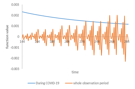
The functions of MSCI_TWI return rate in (11) and (12) are different from the sign of coefficients (-0.6339 and 0.0007), implying different directions of effects on TF return rate when considering different time periods. Besides, the exponential function forms have different signs of the power number. One is XeX and the other is Xe-X, shown in the blue line and the gray line in Figure 5. The functional forms will show whether the contribution of MSCI_TWI return rate to TF return rate converges or diverges, and whether negative MSCI_TWI return rate has more influence on TF return rate.
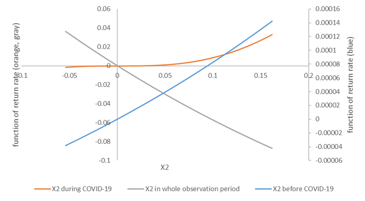
Figure 5. The contributions of the MSCI_TWI return rate on the TF return rate
Figure 5 displays as MSCI_TWI function in (11) occurred a large negative return rate, the function transformation involves a high TF return rate. During the same time period, the contributions of MSCI_TWI functions in (11) and (12) are one-thousandth in difference. Thus, MSCI_TWI can contribute more on the TF return rates in (11). When MSCI_TWI return rates are shifted from negative to positive values, its contributions on the TF return rates become from positive to negative values. But the increase of MSCI_TWI in (12) induces the TF return rate slowly increase from negative to positive values.
|
|
(14) |
|
|
(15) |
The first-order differential from (11) and (12) are (14) and (15), respectively. Displaying in gray line of Figure 5 and (14), negative slope is the negative marginal effect of TF return rate on MSCI_TWI before COVID-19 period (see orange line). Since the MSCI_TWI return rate fell in -0.06 ~ 0.03 before COVID-19 which is less than 1 implies that 1 % increases in the MSCI_TWI return rate resulting in TF return rate decreased.
As for the blue line of Figure 5, (15) implies 1 % increases in the MSCI_TWI return rate inducing the increase of TF return rate. The function form also implies that the MSCI_TWI return rate that took a jump, such as 0.06 or more will lead to the exponential growth of the TF return rate. However, this status did not occur before COVID-19 in Taiwan because the Taiwan security market has the characteristic of “always going up and less going down” and “slowly climbing and fast dropping. (15) also implies that the TF return rate fast decreases and converges to zero as the MSCI_TWI return rate becomes large.
Since the MSCI_TWI return rate affect the TF return rate forming a trigonometric function during COVID-19, the MSCI_TWI rate of return absorbs the periodic effect of time variables and becomes a variable reflecting the characteristics of contract expiration during COVID-19. Since the MSCI_TWI yield is a ratio ranging from -0.1 to 0.08, the MSCI_TWI yield function instead forms an upward curve passing through the origin (see orange line in Figure 5).
3.2.3. The Effect of TAIEX Return Rate on TF Return Rate
The second main finding is the invariability of the function form of TAIEX and its positive coefficient sign. Whatever before, during COVID-19, or the whole observation period, the effects of TAIEX return rate on the TF return rate all have a positive coefficient and the function form of Xe-X. This implies that TF is indeed the financial derivative of TAIEX, so the effect of TAIEX is heavily and directly reflected on the TF return rate. The COVID-19 pandemic cannot have an impact on this relationship. Besides, the coefficients from before COVId-19 to during COVID-19 become large, that is 0.86 to 0.90. However, the function form of Xe-X shows that the negative return rates of TAIEX provide a larger positive value on the TF return rate. The hedging characteristics of TF can be shown here.
First, whatever before or during COVID-19, the values of TAIEX return rate are covered over -0.06 ~ 0.08. the contributions of TAIEX return rate on TF return rate are shown in Figure 6. The almost linear lines show that TF return rate is positively correlated with TAIEX return rate. The positive slope means the TF return rates are up and down simultaneously with the TAIEX return rates at the same day.
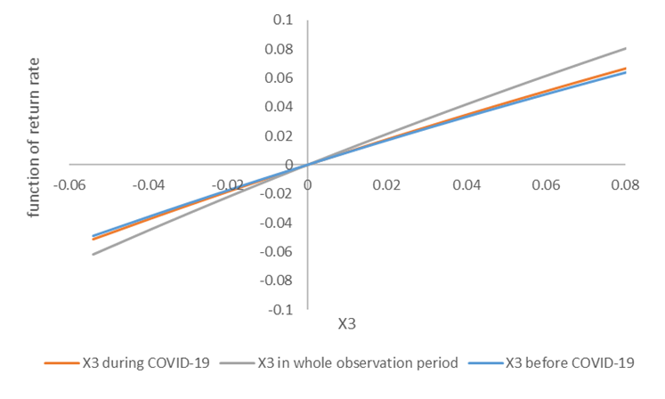
Figure 6. The contributions of the TAIEX return rate on the TF return rate
Figure 6 shows the negative TAIEX return rate leads to the lowest TF return rate as considering the whole observation period (see gray line). The orange line of data during COVID-19 appears in the middle of the three. The three lines are across the original in the figure. This pandemic of COVID-19 induces the relatively higher/lower TF return rates. As given a specific TAIEX return rate (for instance, 0.04), the TF return rate before COVID-19 (on the blue line) is lower than that during COVID-19 (on the orange line). This implies the change of TAIEX return rate brings a higher return rate of TF during COVID-19.
4. Conclusion
This paper has compared the estimated nonlinear model of TF return rate regressed by the time variable, MSCI_TWI return rate, and TAIEX return rate before and during COVID-19. We provided another new analytic direction to investigate stock index futures hit by the shock of COVID-19 pandemic. For the methodology of finding probability distribution for data, it is worth noting that the Laplace distribution is the probability distribution of three kinds of return rates in our study, not Normal distribution. Thus, we select the OLS estimation for the regression analysis, not the MLE estimation. The nonlinear regression with 37 function forms can be used on each explanatory variable and is better than the linear regression that shows the trend of TF return rate. Surprisingly, the time variable can show the oscillation of TF return rates whose values are around zero as analyzing the data of the whole observation period. The positive oscillating values of TF return rate occurred before COVID-19. At the same time, the positive values with downward sloping of TF return rate occurred during COVID-19. The time variable function can show evidence for us how COVID-19 affects the TF return rates. If we consider the data pairs before COVID-19, the time variable can grab the characteristics of the nearby month futures contracts. There are very apparent cycles of futures settlement days.
For the MSCI_TWI return rate that is a kind of financial derivative, the MSCI_TWI return rate plays a different role before and during COVID-19. As considering data of the whole observation period, the functions of MSCI_TWI return rate have different effects on the TF return rate before and during COVID-19. For the TAIEX return rate, the function forms and the sign of coefficients are invariable in the nonlinear estimations. This implies TF is the financial derivative of TAIEX, so they have a strong and stable association. Specially, the TF return rate is positively related with the TAIEX return rate whatever COVID-19 occurs or not.
Finally, this paper provides a methodology of nonlinear regression to investigate the association of the stock index futures and stock price indices and evaluate the effects of stock price indices on the stock index futures. Another methodology of finding the probability distribution for financial data is very important for the MLE estimation and for the artificial intelligence system of Fintech. However, the limitation of this paper is that we do not consider the possibility of arbitrage trading, cross hedging, or volatility. Of course, the data size is too small to cover more information of the stock index futures and other variables. For the future research, we might consider the aim of artificial intelligence system for the stock index futures, which the accurate mathematical estimated model should be built. We also can consider the lagged-time explanatory variables in the model.
Appendix I. The 45 probability distributions
These are the 45 probability distributions for “improved goodness of fit” to test which probability distribution a set of data is following and show in Table I.
Table Ia. List of 45 Probability distributions
| Uniform distribution, X ~ U(a, b) |
|
| Normal distribution, X ~ N(m, s) |
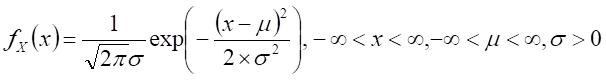
|
|
Shifted exponential distribution,
|
|
| Pareto1 distribution, X ~ Pareto1(λ, c) |
|
| Pareto2 distribution, X ~ Pareto2(λ, c) |
|
| Rayleigh distribution, X ~ Rayleigh(λ, c) |
|
|
Double exponential distribution,
|
|
|
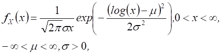
Lognormal distribution
|
|
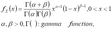
| Gamma distribution, X ~ Gamma(a, b) |
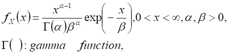
|
| Beta distribution, X ~ Beta (a, b) |
|
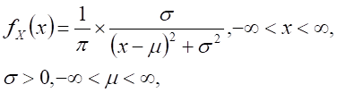
| Cauchy distribution, X ~ Cauchy(m, s) |
|
|
Arcsin distribution,
|
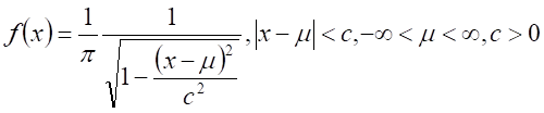
|
|
Gumbel distribution,
|
|
|
Triangular 1 distribution,
|
|
|
Wingner semicircle distribution
|
|
|
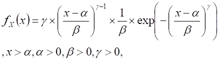
Weibull distribution
|
|
Table Ib. List of 45 Probability distributions (continued)
|
Trapezoid distribution,
|
|
|
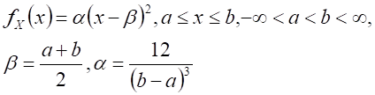
U-quadratic distribution
|
|
|
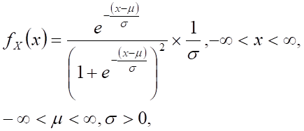
Logistic distribution
|
|
|
Pareto3 distribution
|
|
|
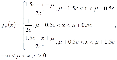
Triangular2 distribution
|
|
|
Triangular3 distribution
|
|
|
Log-logistic distribution
|
|
|
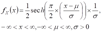
Hyperbolic secant distribution
|
|
|
Kumaraswamy distribution
|
|
|
Gumbel distribution(Type 1)
|
|
|
Gumbel distribution(Type 2)
|
|
Table Ic. List of 45 Probability distributions (continued)
|
Z distribution,
|
|
|
t distribution, |
|
|
Chi square distribution, |
|
| Generalized logistic distribution type I, X ~ G_Logistic(type I)( m, s, a) |
|
| Generalized logistic distribution type II, X ~ G_Logistic(type II)( m, s, a) |
|
| Generalized logistic distribution type III, X ~ G_Logistic(type III)( m, s, a) |
|
|
Generalized normal distribution
|
|
Table Id. List of 45 Probability distributions (continued)
|
Raised cosine distribution
|
|
| Skewed-normal distribution X~Skewed normal distribution(m, s, a) |
|
|
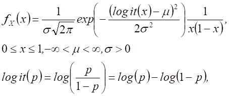
Logit-normal distribution
|
|
|
F distribution, |
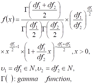
|
| Beta prime distribution |
|
| Bernoulli distribution |
|
| Binomial distribution |
|
| Poisson distribution |
|
| Geometric distribution |
|
| Negative Binomial distribution |
|
| Discrete Uniform distribution |
|
Source: Wang and Lee (2019)
Appendix II. The 37 nonlinear functions
The 37 nonlinear functions of the explanatory variable are summarized below, where X is the explanatory variable and Y is the new explanatory variable after variable transformation by 37 nonlinear function.
Table II. list of 37 functions for the explanatory variable in nonlinear regression
| Y=b0+b1*X | Y=b0+b1*X*Sin(X*pi) |
| Y=b0+b1*X^2 | Y=b0+b1*X*Cos(X*pi)*Cos(X*pi) |
| Y=b0+b1*X^3 | Y=b0+b1*X*Sin(X*pi)*Sin(X*pi) |
| Y=b0+b1*Cos(X*pi) | Y=b0+b1*X*X*Cos(X*pi) |
| Y=b0+b1*Cos(2*X*pi) | Y=b0+b1*X*X*Sin(X*pi) |
| Y=b0+b1*Sin(X*pi) | Y=b0+b1*X*X*Cos(X*pi)*Cos(X*pi) |
| Y=b0+b1*Sin(2*X*pi) | Y=b0+b1*X*X*Sin(X*pi)*Sin(X*pi) |
| Y=b0+b1*Cos(X*pi)*Sin(X*pi) | Y=b0+b1*X*Cos(X*pi)*Sin(X*pi) |
| Y=b0+b1*Cos(X*pi)*Cos(X*pi) | Y=b0+b1*X*X*Cos(X*pi)*Sin(X*pi) |
| Y=b0+b1*Sin(X*pi)*Sin(X*pi) | Y=b0+b1*|X| |
| Y=b0+b1*exp(X) | Y=b0+b1*|X|^0.5 |
| Y=b0+b1*exp(-X) | Y=b0+b1*exp(X)/X |
| Y=b0+b1*log(X) | Y=b0+b1*exp(-X)/X |
| Y=b0+b1/X | Y=b0+b1*exp(X)*log(X) |
| Y=b0+b1*X/(1-X) | Y=b0+b1*exp(-X)*log(X) |
| Y=b0+b1*X*exp(X) | Y=b0+b1*Cos(X) |
| Y=b0+b1*X*exp(-X) | Y=b0+b1*Sin(X) |
| Y=b0+b1*X*Cos(X*pi) | Y=b0+b1*Cos(X)*Cos(X) |
| Y=b0+b1*Sin(X)*Sin(X) |
Source: Wang and Lee (2019)
References
- Chen, L., Li, S., and Wang, J. 2011. Liquidity, skewness and stock returns: evidence from Chinese stock market. Asia-Pacific Financial Markets, 18, pp. 405-427.
- Chen, Y.L., Lee, Y.H., Chou, R.K., and Chang, Y.K., 2021. Arbitrage trading and price discovery of the regular and mini Taiwan stock index futures. Journal of Futures Markets, 41(6), pp. 926-948.
- Fonseca, J.D. and Gottschalk, K., 2013. A Joint Analysis of the Term Structure of Credit Default Swap Spreads and the Implied Volatility Surface. Journal of Futures Markets, 33(6), pp. 494-517.
- Golden, R.M., Henley, S.S., White, H., and Kashner, T.M., 2019. Consequences of model misspecification for maximum likelihood estimation with missing data. Econometrics, 7(3), NO. 37.
- Hull, J. 2003. Options, Futures, and Other Derivative. New Jersey: Prentice-Hall International.
- Johnson, L.L., 1960. The theory of hedging and speculation in commodity futures. Review of Economic Studies, 27, pp. 139-151.
- Jondeau, E., Wang, X.W., Yan, Z.P., and Zhang, Q.Z., 2020. Skewness and index futures return. Journal of Futures Markets, 40(11), pp. 1648-1664.
- Junkus, J.C. and Lee, C.F., 1985. Use of three stock index futures in hedging decisions. Journal of Futures Markets, 5(2), pp. 231-237.
- Mehlitz, J.S. and Auer, B.R., 2021. Time-varying dynamics of expected shortfall in commodity futures markets. Journal of Futures Markets, 41(6), pp. 895-925.
- Park, T.H. and Switzer, L.H., 1995. Time-varying distributions and the optimal hedge ratios for stock index futures. Applied Financial Economics, 5(3), pp. 131-137.
- Tan, X.Y., Wang, C.X., Lin, W., Zhang, J.E., Li, S.H., Zhao, X.J., and Zhang, Z.L., The term structure of the VXX option smirk: Pricing VXX option with a two-factor model and asymmetry jumps. Journal of Futures Markets, 41(4), pp. 439-457.
- Wang, K.S. and Lee, M.Y., 2019. Statistics cannot be the tool of big data analysis-reasons and corrections. Taiwan: Ji-Tong. (In Traditional Chinese Version)
- Yang, J., Li, Z., and Wang, T., 2021. Price discovery in Chinese agricultural futures markets: A comprehensive look. Journal of Futures Markets, 41(4), pp. 536-555.
- Yang, X.L. and Chen, J., 2021. VIX term structure: The role of jump propagation risks. Journal of Futures Markets, 41(6), pp. 785-810.
- Zaremba, A. and Nowak, A., 2015. Skewness preference across countries. Business and Economic Horizons, 11, pp. 115-130.
Article Rights and License
© 2021 The Authors. Published by Sprint Investify. ISSN 2359-7712. This article is licensed under a Creative Commons Attribution 4.0 International License.