Keywordscurrency forwards exchange rate optimization rating migration matrix Risk-free rate risk-free rate modelling
JEL Classification G12
Full Article
1 Introduction
1.1 Fundamentals of Currency Risk
With regards to currency risk, Glick and Rose (1999) emphasize over-valuation, weakness in the banking system, and low international reserves (relative to broad money). The measures that they use are: 1) the annual growth rate of domestic credit, 2) the government budget as a percentage of GDP, 3) the current account as a percentage of GDP, 4) the growth rate of real GDP, 5) the ratio of M2 to international reserves, 6) domestic CPI inflation, and 7) the degree of currency under-valuation.
Frankel and Rose (1996) consider 1) foreign variables like Northern interest rates and output, 2) domestic macroeconomic indicators (output monetary and fiscal shocks), 3) external variables such as over-valuation, 4) the current account and the level of indebtedness, 5) the composition of debt, 6) monetary and fiscal expansions, 7) declining competitiveness, 8) current account deficits, and 9) losses in international reserves. They also note 1) political factors such as political cost of high unemployment or foregone output, 2) the rate of growth of domestic credit, 3) the government budget as a fraction of GDP, 4) the ratio of reserves to imports, 5) the current account as a percentage of GDP, 6) the growth rate of real output, 7) the degree of over-valuation, 8) the measure of international debt (ratio of debt to GNP), 9) vulnerability to external shocks (ratio of foreign exchange reserves to monthly imports; ratio of current account to GDP; real exchange rate), 10) debt composition (foreign direct investment versus portfolio flows; long term versus short term portfolio capital; fixed rate versus floating rate borrowing; domestic versus foreign currency denomination), 11) the amount of concessional debt, and 12) the prospects of rolling over debt. Foreign direct investment versus portfolio investment reflects on the extent that investment contributes to export earnings generation that can service debt, as well as its stability. Global variables include world economic activity, commodity prices, real interest rates, and financial market shocks.
Kaminsky et al (1998) note 105 indicators of currency crises, used in studies, grouped into seven categories: 1) the external sector, 2) the financial sector, 3) the real sector, 4) the public finances, 5) institutional and structural variables, 6) political variables, and 7) contagion effects. They note the indicators are different transformations of the same variable. After consolidation, the following categories emerge: 1) capital account, 2) debt profile, 3) current account; 4) international variables, 5) financial liberalization, 6) other financial variables, 7) real sector, 8) fiscal variables, 9) institutional/ structural factors, and 10) political variables.
Kaminsky et al (1998) argue that authorities abandon exchange rate parity because of concerns of the adverse consequences of policies needed to maintain parity, such as higher interest rates or the level of employment. They emphasize 1) the evolution of the real exchange rate, the current account balance, real wages, domestic interest rates, and foreign interest rates, 2) the relationship between foreign, domestic interest rates and the cost to maintain an exchange rate, 3) the impact of changes in interest rate in response to the exchange rate or the banking sector, 4) the relationship between money supply (purchasing power), and money supply relative to money demand, and exchange rate policy, 5) the relationship between currency appreciation/ value, nominal/ real wages, prices, income, competitiveness, and foreign exchange policy, 6) the fiscal consequences of exchange rate policy, and 7) the strength of the banking system – the proportion of non-performing loans, central bank credit to banks, and a large decline in deposits.
The factors that Corsetti et al (1999) consider are listed in table 1. They further highlight 1) structural distortions: lax supervision and weak regulation, 2) low capital adequacy ratios, 3) lack of incentive-compatible deposit insurance schemes, 4) insufficient expertise in the regulatory institutions, 5) distorted incentives for project selection and monitoring, 6) outright corrupt lending practices, and 7) non-market criteria of credit allocation, according to a model of relationship banking that emphasizes semi-monopolistic relations between banks and firms, somehow downplaying price signals. They also point out the supply-elasticity of foreign funds, and (participant) moral hazard leading to counter-intuitive (investment) action. They focus on the relationship between interest rates, financial system health and stability, and exchange rate stability and depreciation – the relative inability of interest rates to stabilize currencies during crises, particularly with a weak financial system. They also question the impact of capital controls on currency crises (the case for controls on short-term capital inflows; the case for controls on capital outflows in the event of a crisis; and the optimal speed and sequencing of capital account liberalization).
Table 1. Exchange rate risk (Corsetti et al, 1999)
| Current account imbalances and macroeconomic fundamentals | 1) Sustainability of current account imbalances, 2) growth versus total factor productivity growth, with increased investment and labour participation, 3) growth rate expectations, and growth rate shocks, 4) investment rates, (investment) efficiency and (investment) productivity, 5) public and private savings, and the effect of shocks on public savings, and thus sustainability of current account imbalances, 6) domestic to foreign inflation rates and the impact on competitiveness, also in light of the need for seigniorage, 7) openness of the economy, 8) real exchange rate appreciation, 9) political instability and political uncertainty. |
| The financial system | 1) Quantity of financial loans, 2) quality of financial loans, 3) banking problems, 4) financial deregulation and institutional deficiencies. |
| Imbalances in foreign debt accumulation and management | 1) The foreign debt burden and the role of short-term external debt: liquidity, and the ability of foreign reserves to cover debt service obligations, 2) foreign exchange reserves (the stock of reserves in months of imports; the ratio of money assets to foreign reserves; short-term external liabilities), 3) composition and size of capital inflows (volatility of capital sources; currency composition of foreign liabilities). |
1.2 Currency Crises
Frankel and Rose (1996) define a currency crash as a depreciation of the nominal exchange rate of at least 25% that is also at least a 10% increase in the rate of nominal depreciation.
Glick and Rose (1999) note the treatment of currency crises using one of two standard models of speculative attacks: first generation models that focus on inconsistencies between an exchange rate commitment and domestic economic fundamentals, and second generation models that view currency crises as shifts between different monetary policy equilibria in response to self-fulfilling speculative attacks. What is common to both classes of models is their emphasis on macroeconomic and financial fundamentals as determinants of currency crises.
Obstfeld (1996) states that, with second generation models, the focus is on the government’s continuous comparison of the net benefits from changing the exchange rate versus defending it. The coordination problem of currency-market traders changes when changing macroeconomic fundamentals alter the degree of discomfort a government will suffer because of an attack. The state of fundamentals determines the existence and multiplicity of attack equilibria. Fundamentals are neither so strong as to make a successful attack impossible, nor so weak as to make it inevitable. In this case speculators may or may not coordinate on an attack equilibrium. There exists a relationship between fiscal burden and financial sector (banking) pressure, market expectations of depreciation, and domestic interest rates. The central bank may expand the monetary base to function as lender of last resort, and it may put pressure on its foreign reserves. Income distribution, including unexpected interest rate changes redistribute income domestically.
Morris and Shin (1998) note that if speculators believe that a currency will come under attack, their actions in anticipation of this precipitate the crisis itself. On the other hand, if they believe that a currency is not in danger of imminent attack, their inaction spares the currency from attack, thereby vindicating their initial beliefs. Uncertainty about other participants' beliefs is crucial to a speculative episode, since the onset of a speculative attack relies to a large extent on coordinated behavior of speculators. The unique outcome depends on the parameters of the problem, such as the costs of speculation, the underlying strength of the economy, and the size of the pool of hot money in circulation. Information plays a subtle role in speculative crises. What is important is not the amount of information, per se, but rather how public and transparent this information is. If market participants are well informed about the fundamentals, but they are unsure of the information received by other participants, and hence unsure of the beliefs held by others, speculative attacks may be triggered even though everyone knows that the fundamentals are sound. Speculators' beliefs about other speculators' behavior are crucial. Similarly, Corsetti et al (1999) emphasize market overreaction and herding.
Obstfeld (1994) notes that, in addition to reserve adequacy, the effects of high interest rates and growing unemployment help to explain how governments respond to currency crises. If markets expect devaluation, domestic interest rates will rise, thus creating an incentive to devalue. Expectations of devaluation may be incorporated in wage demands, raising authorities' incentive to accommodate. Devaluation expectations may feed into interest rates and can sap government's resolve to resist a validating realignment. Or, expectations may feed into wages and competitiveness, creating similar incentives by raising unemployment.
With regards to currency contagion, Kaminsky et al (1998) argue that contagion can also occur when investors pay little attention to countries' economic fundamentals, and do not discriminate properly between countries. Glick and Rose (1999) note that currency crises tend to be regional, when macroeconomic phenomena do not tend to be regional. On the other hand, trade patterns are regional and can explain why the relevant macro fundamentals are intra-regionally correlated. They propose that currency crises spread along the lines of trade linkages, after accounting for the effects of macroeconomic and financial factors. There are at least two different types of explanations for why contagion spreads - transmission mechanisms that are not mutually exclusive. The first relies on macroeconomic or financial similarity. A crisis may spread from the initial target to another if the two countries share various economic features. The second argues along the lines of trade competitiveness. Countries lose competitiveness when their trading partners devalue, and are likely to devalue themselves.
1.3 Currency Models and Currency Risk
Frankel (1999) notes the two big advantages of fixing the exchange rate are: 1) to reduce transactions costs and exchange rate risk which can discourage trade and investment, and 2) to provide a credible nominal anchor for monetary policy. On the other hand, the big advantage of a floating exchange rate is the ability to pursue an independent monetary policy. Similarly, Alesina and Barro (2000) note two factors that impact sovereign currency policies and currency zones: 1) globalization: the increase in international trade in goods and services, expanded cross-border financial transactions, and heightened cross-country flows of technology, and 2) the increased emphasis on price stability, as opposed to active macroeconomic stabilization, as a goal for monetary policy.
Frankel (1999) argues that, with regards to fixed versus flexible exchange rates, countries have to trade off the advantages of more exchange rate stability against the advantages of more flexibility. However, fixed versus floating is an oversimplified dichotomy. There is in fact a continuum of flexibility, along which it is possible to place most exchange rate arrangements. Currency unions are the firmest commitment to a fixed exchange rate possible. The motivation is to get the maximum credibility for inflation-resistant monetary policy by adopting the strongest commitment. He notes the principle of the impossible trinity: it states that a country must give up one of three goals: exchange rate stability, monetary independence, and financial market integration. An increasingly evident disadvantage of free floating is a tendency toward volatility that does not always derive from macroeconomic fundamentals, including occasional speculative bubbles. Also, an increasingly evident disadvantage of pegging is a tendency toward borrowers’ effectively unhedged exposure in foreign currency, ending badly in speculative attacks and multiple equilibrium. Over-valuation and excessive volatility are possible in either regime. Many of the country characteristics that are most important to the fixed-versus-floating question are closely related to the size and openness of the country.
Alesina and Barro (2000) note that joining a common-currency area can minimize transaction costs and facilitate the flow of information about relative prices, leading to real output and consumption gains. The loss of monetary flexibility has costs and benefits. The country loses a stabilization device targeted to domestic shocks. At the same time, it may gain credibility and thereby reduce undesired inflation. Flexible exchange rates allow monetary independence, but the monetary authorities of many countries lack the ability to commit their policies to a stable and predictable rule. Policies carried out under these conditions may produce high and variable inflation. In addition, it is unclear that monetary discretion is efficiently used in many developing countries to reduce output fluctuations. In this situation, the cost of high inflation is not even compensated by less output variability. Factor mobility and price flexibility are key elements.
Alesina and Barro (2000) further note that, even with a permanently fixed exchange rate, as guaranteed by full dollarization, a country would experience changes in prices relative to those of the anchoring country. These relative price movements reduce the desirability of fixed exchange rates. Therefore, countries would prefer to link to anchors with which they have small variations in relative prices. The determination of optimal currency areas depends on a complex web of variables and interactions, including the size of countries, their ”distance,” the size of the transaction costs of trade, the correlations between shocks, and on institutional arrangements that determine how the seignorage is allocated and whether transfers between members of a union are feasible.
Frankel (1999) notes that countries that are highly integrated with each other, with respect to trade and other economic relationships, are more likely to constitute an optimum currency area. An optimum currency area is a region for which it is optimal to have its own currency and its own monetary policy. An optimum currency area has a optimum size. Optimum currency area criteria include the intensity of trade links and the magnitude of income correlations. The advantages of fixed exchange rates increase with the degree of economic integration, while the advantages of flexible exchange rates diminish. Other factors that may impact the decision to join a monetary union are: the need to satisfy international financial markets and to increase credibility, a desire for closer integration with trading partners, and so forth, and already wide use of the foreign currency.
Frankel and Rose (1998) argue that countries with close international trade links would potentially benefit greatly from a common currency and are more likely to be members of an optimum currency area (OCA). Countries with idiosyncratic business cycles give up a potentially important stabilizing tool if they join a currency union, and countries with symmetric cycles are more likely to be members of an OCA. More importantly, tighter international trade ties may significantly affect the nature of national business cycles. Countries that enter a currency union are likely to experience dramatically different business cycles than before. In part this will necessarily reflect changes in monetary policy; but it will also be a result of closer international trade with the other members of the union. They find that closer international trade links result in more closely correlated business cycles across countries. The high marginal propensity to import associated with an open economy reduces output variability and the need for domestic monetary policy. Openness is one criterion for membership in an OCA. They state four inter-relationships between the members of a potential OCA: 1) the extent of trade; 2) the similarity of the shocks and cycles; 3) the degree of labour mobility; and 4) the system of fiscal transfers (if any). The greater the linkages between the countries using any of the four criteria, the more suitable a common currency.
1.4 Sovereign Risk-Free Rate Modelling
Studies like Brennan and Schwartz (1979), Vasicek (1977), and Cox et al (1985), model the risk-free rate as a single variable, and as a random process. The risk-free rate alone is modelled with few or no independent variables.
To better model sovereign credit risk and currency risk, and to better capture random shifts in the risk-free rate, due to events and shocks, the risk-free rate is allowed to simultaneously migrate between rating categories as risk-free rate ranges, and propagate within rating categories as risk-free rate ranges. A (discrete time, discrete space) Markov process governs the migration between rating categories. When the risk-free rate migrates out of a rating category into another rating category, it leaves a certain risk-free rate range, and enters another risk-free rate range. A random process, like a random walk, governs the propagation within a rating category. While within a particular rating category, the risk-free rate will propagate within the risk-free rate range of the rating category, according to the stipulated random process. This modelling of the risk-free rate falls short of a full blown modelling of the risk free rate as a discrete time, continuous space Markov process, and the use of rating categories simplifies the Markov process, as well as the (specification of the) accompanying Markov kernels.
To practically implement the model, an universal risk-free range is designated – 0% to 100% in this case. A number of rating categories are also designated, and each rating category is assigned a fixed risk-free rate range. The rating categories cover the entire universal risk-free range, with no overlap or gaps between rating categories. The risk-free rate range of each rating category is also made discrete: the risk-free rate range of each rating category is divided by a fixed resolution, such that a number of discrete risk-free rate values or instances are possible within each rating category. An initial (starting) risk-free rate is noted, along with the rating category that it falls in.
During each (discrete time) Markov step, the risk-free rate migrates between rating categories, according to a governing rating migration matrix. With regards to migrating to a rating category, the rule applied is that all discrete risk-free rate instances (values) within the rating category that the risk-free rate migrates to, are equally probable. With regards to propagation within a rating category, the random process used is simply uniform distribution - each discrete risk-free rate instance (value) within the rating category is equally probable. With each Markov step, the probability of each discrete risk-free rate value or instance within each rating category is calculated. Figure 1 depicts the universal risk-free rate range, the rating categories with their risk-free rate ranges, the discrete risk-free rate values within rating categories, as well as both Markov step risk-free rate a) migration out of a rating category and b) propagation within a rating category.
Figure 1. A depiction of risk-free rate a) migration out of a rating category and b) propagation within a rating category
Risk-free rates below 0 are not considered. Also, the state of default is not modelled. It is taken that default is adequately represented by a sufficiently high risk-free rate.
From the probabilities of the risk-free rate instances (values) of the rating categories and the universal risk-free range, and of each discrete time Markov step, the value of a risk-free bond can be determined. The method is further expanded on by Barnard (2019) and Barnard (2017). Equation set 1 stipulates the optimization problem to decompose such a risk-free rate rating migration matrix from market prices. Equation 1.b stipulates the rating migration matrix equality constraint – at all times, the sum of the migration probabilities of each rating category should equal 1. Barnard (2017) details how this constraint can be met during optimization. Equation 1.c and 1.d note additional constraints to guide the solution. Equation 1.c states that for each rating category, the probability of migrating to rating category ![]() must be greater than the probability of migrating to rating category
must be greater than the probability of migrating to rating category ![]() , if rating category
, if rating category ![]() succeeds the particular rating category; and the probability of migrating to rating category
succeeds the particular rating category; and the probability of migrating to rating category ![]() must be greater than the probability of migrating to rating category
must be greater than the probability of migrating to rating category ![]() , if rating category
, if rating category ![]() preceeds the particular rating category. Equation 1.d states that the primary rating category migration probability – the probability of migrating to the same rating category or the probability of remaining in the current rating category – must be greater than a specified minimum value.
preceeds the particular rating category. Equation 1.d states that the primary rating category migration probability – the probability of migrating to the same rating category or the probability of remaining in the current rating category – must be greater than a specified minimum value.
![]() and
and ![]() are the market and modelled bond value of bond
are the market and modelled bond value of bond ![]() , respectively;
, respectively; ![]() is the total number of sample bonds;
is the total number of sample bonds; ![]() is the total number of rating categories;
is the total number of rating categories; ![]() is the probability of migrating from rating category
is the probability of migrating from rating category ![]() to rating category
to rating category ![]() ;
; ![]() is a stipulated floor (minimum) value.
is a stipulated floor (minimum) value.
|
|
(1.a) | |
| Subject to: | ||
|
|
(1.b) | |
|
|
|
(1.c) |
|
|
(1.d) | |
2 Methodology
The purpose of the study is to test the practicality of the proposed risk-free rate model: to what extent a risk-free rate migration matrix can be decomposed and extracted from market data, when assigning a number of risk-free rate rating categories, with risk-free rate ranges, and when assuming migration between the rating categories, and random walks within the rating categories. For this, a simulation is used to source a reference case that can be used for evaluation purposes.
A portfolio of risk-free bonds (representing the same sovereign) is simulated. Each bond has a coupon rate of 7.5, and their maturities are selected such that a span of 20 years is covered, and that each year, a bond matures. This constitutes 20 bonds in total. As shown in table 2, 7 risk-free rate rating categories are used, and their risk-free rate ranges are arbitrarily selected to cover a risk-free rate range from 0% to 100%. A risk-free rate resolution of 1E-04 is used to further sub-divide each rating category. As shown by table 3, a risk-free rate rating migration matrix is simulated. The bond data, rating migration matrix, and risk-free rate rating categories, are used to then calculate prices for the bonds. An initial risk-free rate of 0.06 (6%) is selected, and its corresponding rating category is determined as category BBB. A weekly Markov step interval is used. Figure 2 to 4 show the discount factor, spot rate, and forward rate term structure, respectively, of the simulated risk-free rate rating migration matrix and rating category ranges.
Next, an optimization is run to decompose a risk-free rate rating migration matrix from the simulated bond and price data. The objective is to see how accurately the original migration matrix can again be surfaced. To decompose a rating migration matrix, the method of Barnard (2017) is followed. In all cases, a simple barrier method is used to implement all optimizations. The same method is used to construct an initial solution rating migration matrix that can be further optimized – iteratively optimizing individual rating category migration matrix entries, whilst incrementing a multiplier factor. After an initial solution migration matrix is constructed, it is further optimized by simultaneously or collectively optimizing all rating category migration matrix entries. Barnard (2017) iterates between optimizing rating category migration matrix entries individually, and collectively. But in this case, the bonds comprise a single sovereign and thus a single (initial) rating category. Hence, there is no differentiation between the bonds in terms of rating category, and thus little benefit in optimizing rating category migration matrix entries individually.
Table 2. Simulated risk-free rate rating category risk-free rate regions (0 - 1; 0% - 100%)
| Lower | Upper | |
| AAA | 0.0000 | 0.0180 |
| AA | 0.0180 | 0.0250 |
| A | 0.0250 | 0.0500 |
| BBB | 0.0500 | 0.0800 |
| BB | 0.0800 | 0.1100 |
| B | 0.1100 | 0.1600 |
| CCC | 0.1600 | 1.0000 |
Table 3. Simulated risk-free rate rating category migration matrix
| AAA | AA | A | BBB | BB | B | CCC | |
| AAA | 0.9489 | 0.0273 | 0.0144 | 0.0052 | 0.0025 | 0.0016 | 0.0001 |
| AA | 0.0252 | 0.9155 | 0.0275 | 0.0181 | 0.0072 | 0.0048 | 0.0017 |
| A | 0.0091 | 0.0212 | 0.8854 | 0.0454 | 0.0253 | 0.0082 | 0.0054 |
| BBB | 0.0067 | 0.0198 | 0.0462 | 0.8033 | 0.0638 | 0.0419 | 0.0183 |
| BB | 0.0073 | 0.0284 | 0.0476 | 0.0685 | 0.7417 | 0.0717 | 0.0348 |
| B | 0.0058 | 0.0196 | 0.0337 | 0.0652 | 0.0943 | 0.6833 | 0.0981 |
| CCC | 0.0028 | 0.0084 | 0.0313 | 0.0438 | 0.0876 | 0.1113 | 0.7148 |
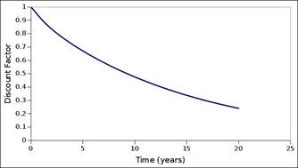
Figure 2. Discount factor term structure of the simulated risk-free rate rating migration matrix and rating category risk-free rate ranges
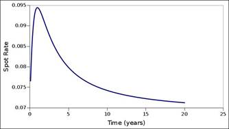
Figure 3. Spot rate term structure of the simulated risk-free rate rating migration matrix and rating category risk-free rate ranges
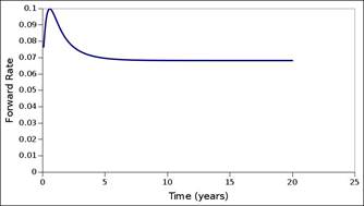
Figure 4. Forward rate term structure of the simulated risk-free rate rating category migration matrix and rating category risk-free rate ranges
3 Analysis
Table 4 shows the decomposed risk-free rate rating migration matrix, when constraint 1.d is omitted, and only constraint 1.c is implemented. The modelling error measures at about 2E-08. What is clear from the matrix is that rating category BBB and B have too low x-to-x migration probabilities – the probability of these rating categories continuing with their respective rating category is too low. Given that the bonds are identical in terms of initial rating, there is little benefit in attempting to optimize the migration matrix entries of these rating categories individually, in the hope that the entries will correct and the x-to-x migration probabilities will increase. The only resolve is to introduce minimum value constraints through constraint 1.d.
Table 4. Decomposed risk-free rate rating migration matrix (iteration 1)
| AAA | AA | A | BBB | BB | B | CCC | |
| AAA | 8.478738e-01 | 1.296161e-01 | 5.919705e-03 | 4.866391e-03 | 3.910231e-03 | 3.908898e-03 | 3.904943e-03 |
| AA | 5.890214e-02 | 9.021574e-01 | 1.248091e-02 | 1.089319e-02 | 7.645239e-03 | 4.288781e-03 | 3.632258e-03 |
| A | 1.904882e-02 | 2.152251e-02 | 8.987143e-01 | 5.808894e-02 | 1.316450e-03 | 1.300590e-03 | 8.353636e-06 |
| BBB | 6.986093e-06 | 6.602035e-04 | 6.805923e-02 | 5.265222e-01 | 3.926772e-01 | 8.163639e-03 | 3.910499e-03 |
| BB | 1.669833e-03 | 1.953609e-03 | 6.203946e-02 | 6.205477e-02 | 8.409458e-01 | 1.568677e-02 | 1.564976e-02 |
| B | 1.555303e-06 | 3.005112e-06 | 2.052011e-02 | 2.367457e-02 | 2.531045e-02 | 4.659770e-01 | 4.645133e-01 |
| CCC | 1.790004e-02 | 2.230670e-02 | 2.456987e-02 | 5.859451e-02 | 6.177172e-02 | 8.011520e-02 | 7.347420e-01 |
Table 5 shows the result when all rating categories' x-to-x migrations are constrained according to the following minimum values: 0.5, 0.5, 0.5, 0.5, 0.5, 0.5, 0.5. The x-to-x migration of rating category BBB and B improved due to this, but are still too low, particularly compared to the x-to-x migration probabilities of neighbour rating categories. There is no significant change in the modelling error.
Table 5. Decomposed risk-free rate rating migration matrix (iteration 2)
| AAA | AA | A | BBB | BB | B | CCC | |
| AAA | 8.689901e-01 | 1.003636e-01 | 1.369698e-02 | 1.008839e-02 | 3.714292e-03 | 2.685761e-03 | 4.615172e-04 |
| AA | 7.152632e-02 | 8.896921e-01 | 1.240000e-02 | 1.184073e-02 | 7.238886e-03 | 6.889536e-03 | 4.124485e-04 |
| A | 8.105092e-04 | 2.756849e-02 | 9.049845e-01 | 4.251318e-02 | 2.248996e-02 | 1.277539e-03 | 3.557945e-04 |
| BBB | 8.801211e-03 | 1.166391e-02 | 6.380198e-02 | 6.024664e-01 | 2.846750e-01 | 2.173828e-02 | 6.853251e-03 |
| BB | 1.024207e-03 | 1.006378e-02 | 5.098444e-02 | 6.722266e-02 | 8.300748e-01 | 2.043766e-02 | 2.019248e-02 |
| B | 1.587120e-06 | 2.366132e-02 | 2.728155e-02 | 5.526186e-02 | 1.153905e-01 | 5.317606e-01 | 2.466425e-01 |
| CCC | 1.213659e-02 | 1.321480e-02 | 1.952168e-02 | 5.441193e-02 | 6.196924e-02 | 6.508274e-02 | 7.736630e-01 |
Table 6 shows the result when all rating categories' x-to-x migrations are constrained according to the following minimum values: 0.5, 0.5, 0.5, 0.5, 0.5, 0.55, 0.5. This still does not provide a satisfactory x-to-x migration probability for rating category BBB and B, and the intuition is to further increase the minimum values. There is no significant change in the modelling error.
Table 6. Decomposed risk-free rate rating migration matrix (iteration 3)
| AAA | AA | A | BBB | BB | B | CCC | |
| AAA | 8.879766e-01 | 8.677836e-02 | 1.109390e-02 | 7.964712e-03 | 2.872274e-03 | 2.190123e-03 | 1.124016e-03 |
| AA | 5.831054e-02 | 8.971202e-01 | 1.997401e-02 | 1.478760e-02 | 7.571723e-03 | 1.376736e-03 | 8.591401e-04 |
| A | 1.721774e-03 | 2.138749e-02 | 9.080024e-01 | 3.460514e-02 | 2.947092e-02 | 3.828633e-03 | 9.836764e-04 |
| BBB | 3.950434e-03 | 1.455747e-02 | 8.177826e-02 | 5.716236e-01 | 3.037321e-01 | 1.253335e-02 | 1.182479e-02 |
| BB | 3.329465e-04 | 1.294177e-02 | 3.766690e-02 | 8.937706e-02 | 8.035337e-01 | 3.659173e-02 | 1.955590e-02 |
| B | 2.237572e-03 | 3.346636e-02 | 4.027648e-02 | 6.000849e-02 | 1.353752e-01 | 5.575342e-01 | 1.711017e-01 |
| CCC | 6.530845e-03 | 2.904372e-02 | 3.122028e-02 | 4.829907e-02 | 5.191296e-02 | 5.193668e-02 | 7.810564e-01 |
Table 7 shows the result when all rating categories' x-to-x migrations are constrained according to the following minimum values: 0.5, 0.5, 0.5, 0.6, 0.5, 0.6, 0.5. The x-to-x migration probability of rating category B has significantly improved at this point. Yet, compared to the x-to-x migration probabilities of its neighbours, it is still low. There is no significant change in the modelling error.
Table 7. Decomposed risk-free rate rating migration matrix (iteration 4)
| AAA | AA | A | BBB | BB | B | CCC | |
| AAA | 8.563221e-01 | 1.260250e-01 | 6.567581e-03 | 5.542303e-03 | 5.541935e-03 | 8.967409e-07 | 1.724652e-07 |
| AA | 7.083860e-02 | 8.791382e-01 | 2.999377e-02 | 9.965464e-03 | 9.886154e-03 | 1.773870e-04 | 4.672431e-07 |
| A | 1.320288e-05 | 2.356602e-02 | 9.057433e-01 | 5.635864e-02 | 6.220952e-03 | 5.049105e-03 | 3.048795e-03 |
| BBB | 1.188977e-02 | 2.445428e-02 | 4.289165e-02 | 6.564549e-01 | 2.358408e-01 | 1.424737e-02 | 1.422131e-02 |
| BB | 4.953656e-03 | 4.958175e-03 | 4.626072e-02 | 5.807183e-02 | 8.256280e-01 | 3.723527e-02 | 2.289232e-02 |
| B | 1.088520e-06 | 1.700733e-02 | 6.306563e-02 | 6.306590e-02 | 1.123291e-01 | 6.312568e-01 | 1.132741e-01 |
| CCC | 1.475968e-06 | 1.318095e-02 | 2.006385e-02 | 5.334962e-02 | 6.420982e-02 | 7.866634e-02 | 7.705280e-01 |
Table 8 shows the result when all rating categories' x-to-x migrations are constrained according to the following minimum values: 0.5, 0.5, 0.5, 0.65, 0.5, 0.65, 0.5. The x-to-x migration probability of rating category B is pressed against the floor or minimum value. It is also evident that the x-to-x migration probability of rating category AAA has now significantly dropped. There is no significant change in the modelling error. The next step is to note the output, when rating category A is constrained to its previous value, before the drop.
Table 8. Decomposed risk-free rate rating migration matrix (iteration 5)
| AAA | AA | A | BBB | BB | B | CCC | |
| AAA | 8.195585e-01 | 1.650813e-01 | 5.136792e-03 | 5.110499e-03 | 5.101164e-03 | 1.013648e-05 | 1.680540e-06 |
| AA | 8.616839e-02 | 8.648757e-01 | 2.427392e-02 | 1.262546e-02 | 8.489371e-03 | 3.267875e-03 | 2.993011e-04 |
| A | 7.614390e-03 | 1.615115e-02 | 9.059401e-01 | 3.191112e-02 | 2.890449e-02 | 8.691557e-03 | 7.871825e-04 |
| BBB | 6.180493e-03 | 1.607081e-02 | 4.434783e-02 | 7.465025e-01 | 1.517438e-01 | 1.757825e-02 | 1.757645e-02 |
| BB | 2.052003e-06 | 7.732845e-03 | 4.307686e-02 | 5.384954e-02 | 8.312372e-01 | 4.165344e-02 | 2.244808e-02 |
| B | 1.007119e-05 | 3.547236e-02 | 4.174562e-02 | 4.174868e-02 | 1.148207e-01 | 6.500183e-01 | 1.161843e-01 |
| CCC | 1.873452e-05 | 3.315845e-02 | 5.043657e-02 | 5.043833e-02 | 5.045387e-02 | 7.560408e-02 | 7.398900e-01 |
Table 9 shows the result when all rating categories' x-to-x migrations are constrained according to the following minimum values: 0.85, 0.5, 0.5, 0.65, 0.5, 0.65, 0.5. The x-to-x migration of rating category AAA recovered, but that of rating category BBB has dropped.
Table 9. Decomposed risk-free rate rating migration matrix (iteration 6)
| AAA | AA | A | BBB | BB | B | CCC | |
| AAA | 8.976375e-01 | 7.708437e-02 | 1.659752e-02 | 4.341097e-03 | 4.339464e-03 | 1.052163e-08 | 6.892328e-09 |
| AA | 5.655749e-02 | 8.962090e-01 | 2.387186e-02 | 1.949523e-02 | 3.169125e-03 | 3.486507e-04 | 3.486342e-04 |
| A | 1.805312e-03 | 1.955614e-02 | 9.044575e-01 | 5.208224e-02 | 1.223880e-02 | 8.482198e-03 | 1.377830e-03 |
| BBB | 1.362089e-02 | 1.362112e-02 | 6.076341e-02 | 6.865574e-01 | 1.911004e-01 | 1.716856e-02 | 1.716827e-02 |
| BB | 9.215108e-05 | 1.666477e-02 | 2.325434e-02 | 6.300889e-02 | 8.260285e-01 | 4.850942e-02 | 2.244197e-02 |
| B | 3.723076e-07 | 2.413821e-02 | 7.413293e-02 | 7.413327e-02 | 7.413339e-02 | 6.541072e-01 | 9.935463e-02 |
| CCC | 1.062153e-07 | 7.435751e-03 | 5.389296e-02 | 5.389339e-02 | 5.389350e-02 | 6.165988e-02 | 7.692244e-01 |
Table 10 shows the result when all rating categories' x-to-x migrations are constrained according to the following minimum values: 0.85, 0.5, 0.5, 0.7, 0.5, 0.65, 0.5. The x-to-x migration of rating category B is still relatively low, and is targeted next.
Table 10. Decomposed risk-free rate rating migration matrix (iteration 7)
| AAA | AA | A | BBB | BB | B | CCC | |
| AAA | 8.817161e-01 | 9.054608e-02 | 1.220090e-02 | 1.219742e-02 | 3.329084e-03 | 8.188071e-06 | 2.208411e-06 |
| AA | 8.336316e-02 | 8.746374e-01 | 1.436972e-02 | 1.436720e-02 | 7.137477e-03 | 3.071722e-03 | 3.053291e-03 |
| A | 1.055283e-05 | 2.700197e-02 | 9.085542e-01 | 4.699518e-02 | 9.380211e-03 | 6.859962e-03 | 1.197911e-03 |
| BBB | 1.484316e-02 | 2.956613e-02 | 2.956614e-02 | 7.656851e-01 | 1.020162e-01 | 4.411814e-02 | 1.420510e-02 |
| BB | 2.760701e-06 | 4.643035e-04 | 4.193103e-02 | 1.030975e-01 | 8.060773e-01 | 2.423307e-02 | 2.419404e-02 |
| B | 2.901094e-05 | 1.136518e-02 | 3.584743e-02 | 8.121892e-02 | 8.125507e-02 | 6.505385e-01 | 1.397459e-01 |
| CCC | 1.325230e-05 | 6.510399e-05 | 3.234393e-02 | 7.082329e-02 | 7.119786e-02 | 7.122534e-02 | 7.543312e-01 |
Table 11 shows the result when all rating categories' x-to-x migrations are constrained according to the following minimum values: 0.85, 0.5, 0.5, 0.7, 0.5, 0.68, 0.5. The x-to-x migration probability of rating category B has improved, but the x-to-x migration probabilities of rating category A, and in particular rating category BB have dropped.
Table 11. Decomposed risk-free rate rating migration matrix (iteration 8)
| AAA | AA | A | BBB | BB | B | CCC | |
| AAA | 9.579051e-01 | 9.468069e-03 | 9.468069e-03 | 5.830628e-03 | 5.830627e-03 | 5.830626e-03 | 5.666849e-03 |
| AA | 5.303775e-02 | 8.860483e-01 | 2.304085e-02 | 2.100581e-02 | 1.212099e-02 | 3.043915e-03 | 1.702427e-03 |
| A | 4.797771e-03 | 7.529776e-02 | 8.623205e-01 | 5.555873e-02 | 6.750898e-04 | 6.750806e-04 | 6.750790e-04 |
| BBB | 3.958529e-11 | 2.460587e-03 | 6.880241e-02 | 8.411221e-01 | 4.896764e-02 | 2.210908e-02 | 1.653822e-02 |
| BB | 1.094950e-10 | 9.273292e-10 | 8.513971e-03 | 6.013922e-02 | 5.033556e-01 | 2.591615e-01 | 1.688297e-01 |
| B | 2.120253e-11 | 1.165026e-02 | 6.638425e-02 | 1.088867e-01 | 1.088867e-01 | 6.995160e-01 | 4.676128e-03 |
| CCC | 5.105330e-12 | 2.331570e-11 | 2.450730e-02 | 5.400891e-02 | 6.370801e-02 | 1.199665e-01 | 7.378092e-01 |
Table 12 shows the result when all rating categories' x-to-x migrations are constrained according to the following minimum values: 0.85, 0.5, 0.5, 0.7, 0.65, 0.68, 0.5. The x-to-x migration probability of rating category A partially corrected, but the x-to-x migration probability of rating category CCC has significantly worsened, and the x-to-x migration probabilities of rating categories AA and A have dropped.
Table 12. Decomposed risk-free rate rating migration matrix (iteration 9)
| AAA | AA | A | BBB | BB | B | CCC | |
| AAA | 9.574512e-01 | 1.139228e-02 | 1.139228e-02 | 4.941064e-03 | 4.941064e-03 | 4.941063e-03 | 4.941062e-03 |
| AA | 6.112125e-02 | 7.806742e-01 | 1.103983e-01 | 4.780632e-02 | 2.705097e-10 | 2.703971e-10 | 8.262653e-12 |
| A | 4.997825e-03 | 1.351426e-01 | 7.957594e-01 | 4.802424e-02 | 5.358646e-03 | 5.358646e-03 | 5.358634e-03 |
| BBB | 6.283606e-10 | 3.560843e-02 | 4.460625e-02 | 8.233802e-01 | 5.011005e-02 | 2.566985e-02 | 2.062523e-02 |
| BB | 2.841690e-09 | 3.281886e-09 | 4.024183e-09 | 3.644338e-02 | 6.500000e-01 | 1.733449e-01 | 1.402117e-01 |
| B | 4.770822e-10 | 1.891816e-02 | 7.205875e-02 | 7.232389e-02 | 7.643834e-02 | 6.800000e-01 | 8.026086e-02 |
| CCC | 2.495009e-06 | 2.519274e-06 | 3.416997e-02 | 1.101687e-01 | 1.101687e-01 | 1.558891e-01 | 5.895985e-01 |
Table 13 shows the result when all rating categories' x-to-x migrations are constrained according to the following minimum values: 0.85, 0.5, 0.5, 0.7, 0.65, 0.68, 0.63. At this point, the x-to-x migration probabilities of rating category AA, A, and BB are still relatively low, compared to neighbours.
Table 13. Decomposed risk-free rate rating migration matrix (iteration 10)
| AAA | AA | A | BBB | BB | B | CCC | |
| AAA | 9.505512e-01 | 2.245759e-02 | 5.398262e-03 | 5.398256e-03 | 5.398247e-03 | 5.398244e-03 | 5.398237e-03 |
| AA | 6.618222e-02 | 7.529061e-01 | 1.636344e-01 | 5.759109e-03 | 5.759105e-03 | 5.759105e-03 | 6.757835e-10 |
| A | 1.107457e-10 | 1.524510e-01 | 7.561424e-01 | 7.109944e-02 | 7.940935e-03 | 7.940933e-03 | 4.425270e-03 |
| BBB | 3.329801e-11 | 7.427712e-03 | 4.237585e-02 | 8.522663e-01 | 5.763122e-02 | 2.014945e-02 | 2.014945e-02 |
| BB | 6.924913e-13 | 9.320580e-11 | 2.625605e-02 | 9.923470e-02 | 6.695358e-01 | 1.454397e-01 | 5.953374e-02 |
| B | 5.090718e-11 | 4.327546e-02 | 5.334570e-02 | 5.334573e-02 | 5.334586e-02 | 7.675177e-01 | 2.916959e-02 |
| CCC | 3.802432e-12 | 9.597776e-11 | 6.989478e-02 | 6.989479e-02 | 6.989480e-02 | 6.989480e-02 | 7.204208e-01 |
Table 14 shows the result when all rating categories' x-to-x migrations are constrained according to the following minimum values: 0.88, 0.85, 0.83, 0.75, 0.7, 0.68, 0.63. At this point it can be argued that the x-to-x migration probability of rating category AA and A are too close to each other, and that that of rating category AAA and AA are too far from each other. At this point, the modelling error is 2.5E-10.
Table 14. Decomposed risk-free rate rating migration matrix (iteration 11)
| AAA | AA | A | BBB | BB | B | CCC | |
| AAA | 9.537696e-01 | 1.462396e-02 | 1.462396e-02 | 4.245862e-03 | 4.245862e-03 | 4.245862e-03 | 4.244948e-03 |
| AA | 4.402664e-02 | 8.606591e-01 | 5.516710e-02 | 1.931207e-02 | 1.530726e-02 | 5.527843e-03 | 1.052516e-09 |
| A | 1.522899e-02 | 5.537049e-02 | 8.668095e-01 | 6.169185e-02 | 8.991211e-04 | 2.102257e-08 | 1.264655e-11 |
| BBB | 5.072903e-11 | 4.402540e-02 | 4.575898e-02 | 7.862103e-01 | 7.831368e-02 | 2.573780e-02 | 1.995382e-02 |
| BB | 7.770477e-10 | 5.207800e-03 | 6.259115e-03 | 6.438777e-02 | 7.478590e-01 | 9.469396e-02 | 8.159233e-02 |
| B | 1.756805e-09 | 1.075741e-02 | 7.183263e-02 | 7.183263e-02 | 7.183264e-02 | 7.360435e-01 | 3.770119e-02 |
| CCC | 1.001704e-10 | 4.345510e-10 | 1.545285e-02 | 4.495502e-02 | 4.920566e-02 | 1.965141e-01 | 6.938724e-01 |
Table 15 notes the difference between the simulated and decomposed rating migration matrix. The simulated rating migration matrix is subtracted from the decomposed rating migration matrix. Negative values imply that the decomposed migration matrix value is higher than the simulated migration matrix value. The greatest x-to-x migration probability error is 0.05484 and occurs for rating category AA. The greatest x-to-y migration probability error is 0.0852 - rating category CCC migrating to rating category B.
Table 15. Difference between the simulated and decomposed rating migration matrix
| AAA | AA | A | BBB | BB | B | C | |
| AAA | −0.0049 | 0.01268 | −0.0002 | 0.00095 | −0.0017 | −0.0026 | −0.0041 |
| AA | −0.0188 | 0.05484 | −0.0277 | −0.0012 | −0.0081 | −0.0007 | 0.0017 |
| A | −0.0061 | −0.0342 | 0.01859 | −0.0163 | 0.0244 | 0.0082 | 0.0054 |
| BBB | 0.0067 | −0.0242 | 0.00044 | 0.01709 | −0.0145 | 0.01616 | −0.0017 |
| BB | 0.0073 | 0.02319 | 0.04134 | 0.00411 | −0.0062 | −0.023 | −0.0468 |
| B | 0.0058 | 0.00884 | −0.0381 | −0.0066 | 0.02247 | −0.0527 | 0.0604 |
| CCC | 0.0028 | 0.0084 | 0.01585 | −0.0012 | 0.03839 | −0.0852 | 0.02093 |
4 Conclusion
The decomposed risk-free rate rating migration matrix is generally accurate, when the appropriate constraints are used to guide the decomposition. This suggests that it will also be possible to decompose such a migration matrix from market data, with appropriate accuracy.
The model lets the risk-free rate simultaneously migrate between rating categories as risk-free rate ranges, and propagate within rating categories as risk-free rate ranges. This is seen to better model the true nature of the risk-free rate, and to better allow for random shifts in the risk-free rate, relaying distinct events and shocks. The use of rating categories as risk-free rate ranges simultaneously enriches and simplifies the modelling of the risk-free rate. The risk-free rate model greatly infers and builds on the relationship between the current risk-free rate and likely future risk-free rates, and the current risk-free rate and risk-free rate volatility. By clustering risk-free rates into risk-free rate categories, it is presumed that comparable risk-free rates demonstrate similar properties – most notably risk-free rate volatility and migration (future risk-free rate) probabilities. Sovereign credit ratings should then also infer certain properties with regards to risk-free rate ranges and risk-free rate volatility. It also postulates that sovereign credit ratings are or should be comparable and universal.
The study arbitrarily assigned rating categories, and arbitrarily assigned risk-free rate ranges to these rating categories. The basic requirement is that the risk-free rate properties of risk-free rate instances within a rating category are comparable. Empirical research can further examine and clarify this, and delineate likely rating categories and risk-free rate ranges, by further examining the relationship between the risk-free rate and risk-free rate volatility. Comparable risk-free rates should illustrate comparable risk-free rate volatility, and risk-free rates should cluster in terms of their risk-free rate volatility characteristics. Also, empirical research can examine the risk-free rate range and risk-free rate volatility properties of sovereign credit ratings.
A benefit of the risk-free rate model is that it is entirely ahistorical. Also, future risk-free rate probability distributions can easily be generated by the model. This has particular benefits for exchange rate – currency forwards – valuation. Further refinements to the model are possible, particularly in terms of the process and rules of migration out of a rating category into another rating category, and propagation within rating categories. The model mostly utilized uniform distribution - equal probabilities - and future models can consider more sophisticated processes and rules.
References
- Alesina, A. and Barro, R.J., 2000. Currency unions (No. w7927). National Bureau of Economic Research.
- Barnard, B., 2017. Rating Migration and Bond Valuation: Decomposing Rating Migration Matrices from Market Data via Default Probability Term Structures. Expert Journal of Finance, 5, pp. 49-72.
- Barnard, B., 2019. Rating Migration and Bond Valuation: Towards Ahistorical Rating Migration Matrices and Default Probability Term Structures. Applied Finance and Accounting, 5(1), pp. 12-41.
- Brennan, M.J. and Schwartz, E.S., 1979. A continuous time approach to the pricing of bonds. Journal of Banking & Finance, 3(2), pp.133-155.
- Corsetti, G., Pesenti, P. and Roubini, N., 1999. What caused the Asian currency and financial crisis?. Japan and the world economy, 11(3), pp.305-373.
- Cox, J.C., Ingersoll Jr, J.E. and Ross, S.A., 1985. A theory of the term structure of interest rates. Econometrica: Journal of the Econometric Society, pp.385-407.
- Frankel, J.A. and Rose, A.K., 1996. Currency crashes in emerging markets: An empirical treatment. Journal of international Economics, 41(3), pp.351-366.
- Frankel, J.A. and Rose, A.K., 1998. The endogenity of the optimum currency area criteria. The Economic Journal, 108(449), pp.1009-1025.
- Frankel, J.A., 1999. No single currency regime is right for all countries or at all times (No. w7338). National Bureau of Economic Research.
- Glick, R. and Rose, A.K., 1999. Contagion and trade: Why are currency crises regional?. Journal of international Money and Finance, 18(4), pp.603-617.
- Kaminsky, G., Lizondo, S. and Reinhart, C.M., 1998. Leading indicators of currency crises. Staff Papers, 45(1), pp.1-48.
- Morris, S. and Shin, H.S., 1998. Unique equilibrium in a model of self-fulfilling currency attacks. American Economic Review, pp.587-597.
- Obstfeld, M., 1994. The logic of currency crises (No. w4640). National Bureau of Economic Research.
- Obstfeld, M., 1996. Models of currency crises with self-fulfilling features. European economic review, 40(3), pp.1037-1047.
- Vasicek, O., 1977. An equilibrium characterization of the term structure. Journal of financial economics, 5(2), pp.177-188.
Article Rights and License
© 2019 The Author. Published by Sprint Investify. ISSN 2359-7712. This article is licensed under a Creative Commons Attribution 4.0 International License.