Keywordsconsumption-leisure choice income elasticity of demand money illusion propensity to search Veblen effect
JEL Classification D11, D83
Full Article
1. Introduction
The analysis of the optimal consumption-leisure choice under price dispersion discovers the behavioral importance of the propensity to search, i.e., of the willingness to substitute labor by search for advantageous prices (Malakhov 2015). While modest propensity to search creates a “common model” of behavior where the search displaces both labor and leisure time in the time horizon like ice displaces whiskey and soda in the glass, the vigorous propensity to search reduces labor time for both search and leisure time and results in either “labor” or “leisure” model of behavior. However, the propensity to search goes far beyond the models of allocation of time. This key variable of the optimal search model significantly affects the structure of consumption under price dispersion.
While effects of the propensity to search on consumption pattern are so important, this paper is organized as follows. Part 2 confirms the identity of marginal utilities of both consumption and leisure in the classical individual labor supply model and in the “common model” of optimal search. This conclusion approves the methodological reliability of the model of optimal search. Part 3 describes the mechanism of the vigorous propensity to search that results in “labor” and “leisure” model. These models correspond to the classical backward-bending curve under classical individual labor supply. There, marginal utilities loose its identity because in the search model either consumption or leisure gets the negative marginal utility. Part 4 analyses the wage elasticity of the propensity to search. And this analysis discovers the fact that the “common model”, which is identical to the classical model of the individual supply, results in normal wage inelastic demand, while the wage elastic demand occurs under either “labor” or “leisure” model of behavior where one of key variables, either consumption or leisure, becomes “bad” with negative marginal utility. The assumption that elastic demand is formed by “the leisure model” is followed by the step-by-step appearance of the money illusion. Part 5 proposes some methodological conclusions like the analysis of the equilibrium with “bads” and discovers the need in detail studies of income elasticity for consumption, labor, and leisure.
2. Identity of Marginal Utilities in the “Common Model” Under Price Dispersion and in the Classical Model of the Individual Labor Supply
If we denote labor time as ![]() , leisure time as
, leisure time as ![]() , and the time of search for the interesting price as
, and the time of search for the interesting price as ![]() , where the time horizon
, where the time horizon ![]() until the next purchase is equal to
until the next purchase is equal to ![]() ,
, ![]() as the wage rate and
as the wage rate and ![]() as consumption, we can modify the famous G.Stigler’s equation of the optimal search (Stigler 1961) and use it as the constraint to the problem of the maximization of consumption-leisure utility function
as consumption, we can modify the famous G.Stigler’s equation of the optimal search (Stigler 1961) and use it as the constraint to the problem of the maximization of consumption-leisure utility function ![]() . The store when a consumer finds the interesting price can be presented bt the value of marginal decrease in the price of purchase
. The store when a consumer finds the interesting price can be presented bt the value of marginal decrease in the price of purchase ![]() . The value of marginal savings on purchase or the marginal benefit on search is equal to
. The value of marginal savings on purchase or the marginal benefit on search is equal to ![]() . The consumer finds the advantageous price and tries to optimize the quantity to be purchased with leisure time. Here he is constrained by the equality of marginal savings with the marginal loss in labor income. While labor and search represent alternative sources of income, we get the value of the propensity to search
. The consumer finds the advantageous price and tries to optimize the quantity to be purchased with leisure time. Here he is constrained by the equality of marginal savings with the marginal loss in labor income. While labor and search represent alternative sources of income, we get the value of the propensity to search ![]() and the marginal loss is equal to the value
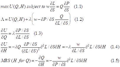
and the marginal loss is equal to the value ![]() . The equality of the marginal loss to the marginal benefit gives us the constraint for the maximization of the consumption-leisure utility (Equations 1.1-1.5)
. The equality of the marginal loss to the marginal benefit gives us the constraint for the maximization of the consumption-leisure utility (Equations 1.1-1.5)
When ![]() , we have for the given time horizon:
, we have for the given time horizon:
![]() (2)
(2)
The Equation (2) gives us a possibility to choose the following Cobb-Douglas utility function:
![]() (3)
(3)
The graphical presentation confirms the idea that the search displaces in the time horizon both labor and leisure like ice displaces both whiskey and soda in the glass. We denote this metaphor as “the common model” of behavior. Supported by the graphical analysis (Fig.1), this metaphor gives us the value of the propensity to search:
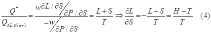
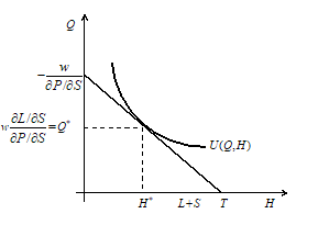
Figure 1. “Common model” of behavior
From here we can simplify the presentation of the unusual marginal values given in Equations 1.1-1.5. First, we can re-write the second-order derivative ![]() :
:
![]()
Then, we can confirm our assumption that the given utility curve comes from the family of Cobb-Douglas utility functions:
The transformation of the budget constraint comes to the assumption that the equilibrium price is equal to the value of total costs of purchase of one unit of consumption ![]() :
:
Then, the marginal values of both consumption and leisure take the following forms:
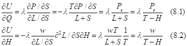
If we try to determine the value of the Lagrangian multiplier for the problem we get (Malakhov 2015)
![]()
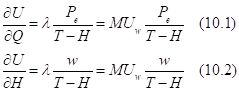
The values of marginal utilities take the following forms:
The Lagrangian multiplier in the classical consumption-leisure choice under labor-leisure trade-off is equal to (Baxley and Moorhouse 1994):
![]()
Then, the classical optimal consumption-leisure choice under the labor-leisure trade-off comes to the following values:
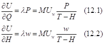
We see that the optimal consumption-leisure choice under price dispersion is identical to the optimal consumption-leisure choice under the classical labor-leisure trade-off.
However, it is true only for the common model of behavior where “ice-whiskey-soda” metaphor works. The value of the propensity to search in the “common model” is limited by:
![]()
We can re-arrange the budget constraint for the corner solution where ![]() :
:
![]()
However, when the wage rate is less than the absolute value of marginal savings, the consumer cannot buy the quantity demanded even in the corner because he has chosen the item on the market where marginal savings on purchase are greater than the wage rate, or ![]() :
:
![]()
To buy the quantity demanded the consumer needs the great propensity to search, or ![]() and
and ![]() .
.
Now we find the roots of the vigorous propensity to search. The consumer needs it when marginal savings on a particular market are greater than his wage rate.
3. Propensity to Search in “Labor” and “Leisure” Models of Behavior
When the absolute value of the propensity to search is greater then one, i.e., ![]() and
and ![]() , the consumer meets the deficit of labor time for purchase, the deficit of search time to find interesting price, and, evidently, the deficit of leisure time to consume. In general, it looks like the deficit of the time horizon (Fig.2):
, the consumer meets the deficit of labor time for purchase, the deficit of search time to find interesting price, and, evidently, the deficit of leisure time to consume. In general, it looks like the deficit of the time horizon (Fig.2):
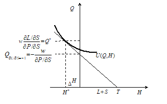
Figure 2. The deficit of leisure
But this picture is really hypothetical. The vigorous propensity to search makes the leisure-search relation positive, or ![]() due to
due to ![]() rule. However, the positive
rule. However, the positive ![]() value changes the sign of the second derivative
value changes the sign of the second derivative ![]() . It becomes negative. An increase in leisure time rises the absolute value of the propensity to search
. It becomes negative. An increase in leisure time rises the absolute value of the propensity to search ![]() and decreases its negative real value
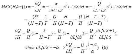
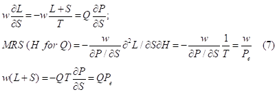
and decreases its negative real value ![]() . The time horizon really becomes negative. But the negative value of the time horizon changes the sign of the marginal utility of leisure (Equation 1.4). It becomes negative. It means that the leisure becomes “bad”. However, the change in the sign of the marginal utility of leisure changes the sign of the MRS (H for Q) in Equation (7). The consumption-leisure relationship becomes positive, or
. The time horizon really becomes negative. But the negative value of the time horizon changes the sign of the marginal utility of leisure (Equation 1.4). It becomes negative. It means that the leisure becomes “bad”. However, the change in the sign of the marginal utility of leisure changes the sign of the MRS (H for Q) in Equation (7). The consumption-leisure relationship becomes positive, or ![]() .
.
We should change axis in order to get the graphical presentation of “bad” leisure (Fig.3):
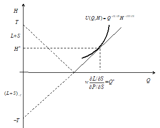
Figure 3. Normal consumption and “bad” leisure
It looks like the consumer has accumulated in the previous time period (![]() is negative) some labor income and some knowledge about an item to be purchased
is negative) some labor income and some knowledge about an item to be purchased![]() But it is not enough to buy the quantity demanded. He continues to work and to search in the current period but he also starts to enjoy the purchase during leisure time.
But it is not enough to buy the quantity demanded. He continues to work and to search in the current period but he also starts to enjoy the purchase during leisure time.
However, we can come back to tradition presentation of the consumption-leisure choice. But this traditional presentation results in normal leisure and “bad” consumption (Fig.4):
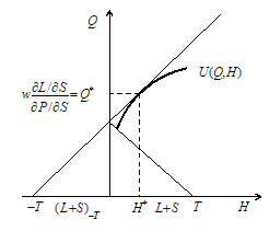
Figure 4. “Bad” consumption and normal leisure
This situation can take place if the Lagrangian multiplier ![]() . Indeed, when
. Indeed, when ![]() , the labor becomes uninteresting with regard to very efficient search. Here again we meet positive consumption-leisure relationship
, the labor becomes uninteresting with regard to very efficient search. Here again we meet positive consumption-leisure relationship ![]() .
.
It is very useful to present the general rule for the optimal level of consumption, which is true not only for all three models of behavior but also for the hypothetical choice under the deficit of leisure (Equation 16):
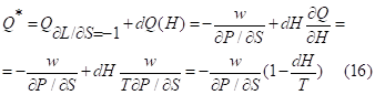
We denote the normal consumption – “bad” leisure relationship as the “labor model” of behavior and the “bad” consumption – normal leisure as the “leisure model” of behavior.
These both models have many common features. First, both models are produced by ![]() relationship that results in the great absolute propensity to search
relationship that results in the great absolute propensity to search ![]() . It takes place when the consumer enters the market where great price reductions are possible. Under the classical assumption of the diminishing efficiency of search
. It takes place when the consumer enters the market where great price reductions are possible. Under the classical assumption of the diminishing efficiency of search ![]() it means that great discounts corresponds to high prices. The situation looks like the consumer enters some new upper price niche that needs more time to work for the purchase, to search, and to enjoy the item to be purchased. Here, the consumer can use the income gained in the previous consumption period and the knowledge from previous searches. But the negative time horizon means that in the previous period the consumer has missed the consumption itself. For example, the bottle of good wine might be the perfect complement for a dinner, but the bottle of good wine doesn’t accompany all dinners. Sometimes dinners are served by vin de table. When the consumer decides to by a good wine in the current period, he gets money from the pocket, he remembers some information from the wine’s guide which he has read before-yesterday, he adds to this “capital” some labor and search time, he buys some bottles of good wine, enjoys it with the dinner, and makes stock for future consumption.
it means that great discounts corresponds to high prices. The situation looks like the consumer enters some new upper price niche that needs more time to work for the purchase, to search, and to enjoy the item to be purchased. Here, the consumer can use the income gained in the previous consumption period and the knowledge from previous searches. But the negative time horizon means that in the previous period the consumer has missed the consumption itself. For example, the bottle of good wine might be the perfect complement for a dinner, but the bottle of good wine doesn’t accompany all dinners. Sometimes dinners are served by vin de table. When the consumer decides to by a good wine in the current period, he gets money from the pocket, he remembers some information from the wine’s guide which he has read before-yesterday, he adds to this “capital” some labor and search time, he buys some bottles of good wine, enjoys it with the dinner, and makes stock for future consumption.
Here we come to the assumption that the negative time horizon means the substitution of the item to be purchased in the current period by some other good. For example, we use bus and train before we buy a car. A qualified medical treatment of grippe could be substituted in old days by whiskey-for-the-night. Other words, the negative time horizon can be treated as a time period when the consumer misses the enjoyment of the desired item. The desired item is consuming irregularly.
Finally, both “labor” and “leisure” models produce the positive consumption-leisure relationship ![]() . This positive relationship comes from the great propensity to search where the consumer cuts labor time in order to increase both search and leisure time
. This positive relationship comes from the great propensity to search where the consumer cuts labor time in order to increase both search and leisure time ![]() .
.
However, there are two important differences between “labor” and “leisure” models.
First, normal consumption – “bad” leisure relationship results in the increase in the intensity of consumption. The “bad” leisure only follows the normal consumption and the increase in its intensity reduces the negative effect of “bad” leisure. Here we simply “kill” the time. Contrarily, the “bad” consumption – normal leisure relationship results in the decrease in the intensity of consumption. Here we simply “fill” the time. The increase in leisure time decreases the negative effect of “bad” consumption.
Second, the behavior under “labor model” is not interesting in great price discounts. There, high prices with great price discounts reduce the utility because marginal savings produce the disutility (Equation 17.2 from Malakhov 2015)
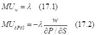
However, when the value of the marginal utility of wage rate ![]() is negative, the increase in wage rate decreases the utility. The utility can be raised only in upper price niche with the increase of the absolute value
is negative, the increase in wage rate decreases the utility. The utility can be raised only in upper price niche with the increase of the absolute value ![]() and the decrease in the real value of price reduction
and the decrease in the real value of price reduction ![]() . The “leisure model” is efficient only with the change of the price niche. Here the Veblen effect takes place. When the consumer enters the new price niche he should spend some search time to understand new prices. But, accompanied by positive
. The “leisure model” is efficient only with the change of the price niche. Here the Veblen effect takes place. When the consumer enters the new price niche he should spend some search time to understand new prices. But, accompanied by positive ![]() and
and ![]() relationship this additional search increases consumption with new high prices:
relationship this additional search increases consumption with new high prices:
![]()
The answer to question whether both “labor” and “leisure” models are widespread lies in the detailed field analysis of the allocation of time. For example, the data from the research of Aguiar and Hurst (2007) gives grounds for the assumption that during last decades of the XX century American women followed the “common model” of behavior while American men exposed either “labor” or “leisure” models of behavior (Malakhov 2015). However, some analytical tools can provide with a quick answer to this question. The solution comes from the analysis of the income elasticity of demand.
4. Income Elasticity of the Propensity to Search
We can present the budget constraint (Equation 1.1) in the form of elasticity with respect to the wage rate for the given price reduction (![]() ). (Here we can simplify the presentation by the absolute values because it is more difficult to understand the elasticity of negative values.)
). (Here we can simplify the presentation by the absolute values because it is more difficult to understand the elasticity of negative values.)
![]()
Now we come back to the “common model” of behavior with modest (![]() ) propensity to search:
) propensity to search:
![]()
We take the simple elasticity of the propensity to search with regard to the wage rate:
The increase in wage rate changes the allocation of time and we get the value of the derivative of the propensity to search:
Indeed, the increase in wage rate makes the search less interesting (![]() ). The decrease in the time search increases labor time because labor becomes more interesting (
). The decrease in the time search increases labor time because labor becomes more interesting (![]() ) and it also rise leisure time because leisure is a normal good (
) and it also rise leisure time because leisure is a normal good (![]() ). This consideration gives us the sign of the wage elasticity of propensity to search:
). This consideration gives us the sign of the wage elasticity of propensity to search:
However, when the elasticity of the absolute value of the propensity to search is negative, the wage rate elasticity of consumption becomes low:
![]()
It means that under the “common model” of behavior the demand is normal but wage inelastic. Moreover, when the wage elasticity of labor supply is positive, and we have this effect in the “common model”, the demand becomes very income inelastic:
![]()
However, if the consumer chooses the upper price niche after the increase in wage rate, he can change brands and quality, for example, the absolute value of marginal savings is also rising, i.e., ![]() (Malakhov 2014), the income elasticity of consumption itself falls again. Coming back to the Equation (19), we can re-write illustratively the Equation (24) in the following manner:
(Malakhov 2014), the income elasticity of consumption itself falls again. Coming back to the Equation (19), we can re-write illustratively the Equation (24) in the following manner:
![]()
We see that the key variable that decreases the wage elasticity of the propensity to search is the diminishing value of the sum of labor and search time ![]() . If we presuppose that it is rising with the wage rate due to the significant increase in labor time
. If we presuppose that it is rising with the wage rate due to the significant increase in labor time ![]() , we should agree with the decrease in leisure time
, we should agree with the decrease in leisure time ![]() . But it means that at the new wage rate level labor substitutes both search and leisure time. Other words, the variables
. But it means that at the new wage rate level labor substitutes both search and leisure time. Other words, the variables ![]() and
and ![]() move in the same direction, or
move in the same direction, or ![]() . It means that we quit “the common model” and we cannot use the Equation (4) for the analysis of the propensity to search. We come to the vigorous propensity to search
. It means that we quit “the common model” and we cannot use the Equation (4) for the analysis of the propensity to search. We come to the vigorous propensity to search ![]() under either “labor” or “leisure” model of behavior. If the consumer increases labor supply with regard to the increase in wage rate, we can present this choice as
under either “labor” or “leisure” model of behavior. If the consumer increases labor supply with regard to the increase in wage rate, we can present this choice as ![]() . If
. If ![]() , this is the “common model” because
, this is the “common model” because ![]() and
and ![]() . If
. If ![]() , this is the “labor model” because
, this is the “labor model” because ![]() and
and ![]() . However, when the market is perfect and S=0, the increase in labor time keeps the income elastic demand within the “common model” because there
. However, when the market is perfect and S=0, the increase in labor time keeps the income elastic demand within the “common model” because there ![]() .
.
Now let’s pay attention to the value of the vigorous propensity to search ![]() . The graphical analysis of both “labor” and “leisure” models gives us the same value of the propensity to search for both models:
. The graphical analysis of both “labor” and “leisure” models gives us the same value of the propensity to search for both models:
![]()
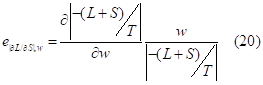
The wage elasticity of the propensity to search takes the following form:
When the increase in the wage rate rises leisure time (dH(w)>0) we have:
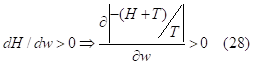
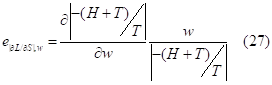
As a result, we get the positive value for the wage elasticity of the absolute value of the propensity to search:
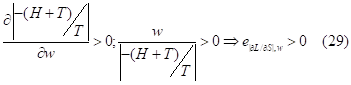
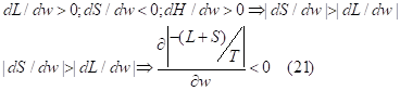
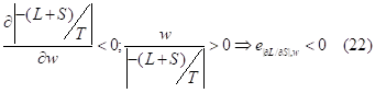
However, the positive wage elasticity of leisure (![]() ) needs more attention. The wage elasticity of leisure is definitely positive in the “leisure model” because there the leisure is a normal good. It is not true for the “labor model” of behavior where leisure is an inferior good. And the consumer can decrease it with the increase in the wage rate. In this case, the wage elasticity of the propensity to search becomes negative and the demand becomes income inelastic. However, here the consumer misses time to consume the increased purchased quantity and he should increase even “bad” leisure in order to enjoy the increased consumption due to the
) needs more attention. The wage elasticity of leisure is definitely positive in the “leisure model” because there the leisure is a normal good. It is not true for the “labor model” of behavior where leisure is an inferior good. And the consumer can decrease it with the increase in the wage rate. In this case, the wage elasticity of the propensity to search becomes negative and the demand becomes income inelastic. However, here the consumer misses time to consume the increased purchased quantity and he should increase even “bad” leisure in order to enjoy the increased consumption due to the ![]() rule that holds in “the labor model”. In this case the wage elasticity of the propensity to search becomes positive again. But for the positive wage elasticity of the propensity to search we get an elastic demand:
rule that holds in “the labor model”. In this case the wage elasticity of the propensity to search becomes positive again. But for the positive wage elasticity of the propensity to search we get an elastic demand:
![]()
Moreover, when the wage elasticity of labor supply is negative ![]() ), and both “labor” and “leisure” models demonstrate the decrease in labor time in favor of both search and leisure, we have:
), and both “labor” and “leisure” models demonstrate the decrease in labor time in favor of both search and leisure, we have:
![]()
However, the change in the price niche weakens again the income elasticity of consumption:
![]()
Evidently, the increase in labor income rises both consumption and leisure but the consumption-leisure relationship for income elastic demand is positive, or
![]()
As we see, the income elastic demand becomes the evident feature of the positive consumption-leisure relationship ![]() . Here we cannot definitely say whether income-elastic demand displays the “leisure” or the “labor” model but for the both models this positive relationship holds.
. Here we cannot definitely say whether income-elastic demand displays the “leisure” or the “labor” model but for the both models this positive relationship holds.
The “bad” nature of income elastic demand can be demonstrated in the other way. The Equation (7) exhibits the transformation of the equations of marginal values of search into the equilibrium price. The equilibrium price under the “common model” is equal to the total costs of purchase ![]() of one unit
of one unit ![]() . But it is not true for both “labor” and “leisure” models. There, consumers spend on purchase labor and search not only in the current period but they also use labor and search accumulated in the previous period. But we don’t definitely know how the previous time horizon has been allocate between labor and search. The only thing we know that the (
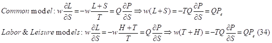
. But it is not true for both “labor” and “leisure” models. There, consumers spend on purchase labor and search not only in the current period but they also use labor and search accumulated in the previous period. But we don’t definitely know how the previous time horizon has been allocate between labor and search. The only thing we know that the (![]() ) value means the time of missed consumption. In addition, if the consumer is willing to sell the purchased elastic item he adds to its price the leisure time, which will be missed in the current time horizon. If in the “common model” the equilibrium price is equal to total costs per unit of purchase, i.e., to the marginal costs on purchase, in both “labor” and “leisure” models we do not find labor and search costs in the equilibrium price. There, the willingness to accept or to sell is equal to the costs of missed leisure. Other words, the equilibrium price is equal to the marginal costs of missed enjoyment from the purchased item (Equation 34):
) value means the time of missed consumption. In addition, if the consumer is willing to sell the purchased elastic item he adds to its price the leisure time, which will be missed in the current time horizon. If in the “common model” the equilibrium price is equal to total costs per unit of purchase, i.e., to the marginal costs on purchase, in both “labor” and “leisure” models we do not find labor and search costs in the equilibrium price. There, the willingness to accept or to sell is equal to the costs of missed leisure. Other words, the equilibrium price is equal to the marginal costs of missed enjoyment from the purchased item (Equation 34):
This is the reasoning for high income elasticity of consumption under both “labor” and “leisure” models. As we have seen, the negative time horizon means that consumers miss in this period the consumption of the desired item. This item is consuming irregularly. But when the chance to buy this item appears consumers are trying to compensate the deficit of consumption in the previous period. They are purchasing more. So, the income elasticity is rising. And it becomes more evident when the elasticity of consumption is calculated indirectly, i.e., on the basis of the expenditures with regard to the income. Here, the accelerated growth rate of expenditures on some item is treated like high income elasticity.
It looks more promising to explain high income elasticity of consumption by the “labor model”, when consumers should increase “bad” leisure in order to provide the consumption growth by additional time. If we try to explain income elasticity by “the leisure model” of behavior we meet a serious problem.
Indeed, the increase in wage rate, other things being equal, decreases the utility level due to the negative marginal utility of labor income ![]() even if the consumer increases the normal leisure time and reduces the inferior consumption. However, the graphical analysis displays the unrealism of that scenario. The budget constraint line becomes steeper after the increase in the wage rate. And it is impossible to increase leisure without the consumption growth. Nevertheless, the decline in utility level under the Equation (17.1) happens (Fig. 5). The consumer feels frustrated.
even if the consumer increases the normal leisure time and reduces the inferior consumption. However, the graphical analysis displays the unrealism of that scenario. The budget constraint line becomes steeper after the increase in the wage rate. And it is impossible to increase leisure without the consumption growth. Nevertheless, the decline in utility level under the Equation (17.1) happens (Fig. 5). The consumer feels frustrated.
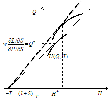
Figure 5. The decrease of utility in “leisure model” after the increase in the wage rate
However, the frustration from the decrease in utility is immediately eliminated by the change in the price niche. The consumer goes to the high-price store where he can restore the utility level. But even if consumer finds the price discounts that correspond to the new wage rate and comes back to the original budget constraint line (![]() ) he does not return to the original utility level. Moreover, this comeback raises the utility level (Fig. 6):
) he does not return to the original utility level. Moreover, this comeback raises the utility level (Fig. 6):
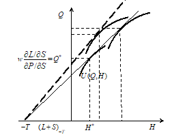
Figure 6.Money illusion in “the leisure model”
The visit to the high-price store raises both consumption and leisure. It happens because the Veblen effect appears (Equation 18). The consumer increases the time of search because he needs more time to understand new prices (![]() ). This increase in search is followed by the increase in leisure time (
). This increase in search is followed by the increase in leisure time (![]() ), and with the positive consumption-leisure relationship (
), and with the positive consumption-leisure relationship (![]() ) it also raises the consumption level (
) it also raises the consumption level (![]() ).
).
We see that when increase in the wage rate and voluntary increase in purchase prices are separated in time both these effects raise successively leisure as well as consumption. The money illusion occurs.
5. Conclusion
The assumption of income inelastic demand in the “common model” is followed by the question what happens with the total disposable income, which should be unit elastic. The consumer should complement the inelastic demand by some elastic item in order to spend the total disposable income. The answer is very simple. The model of the optimal consumption-leisure choice under price dispersion is based on the assumption that the optimal allocation of time for the given consumption level maximizes the reserve for future purchases ![]() (Malakhov 2014b). When consumer maximizes the nonmonetary utility he also maximizes this reserve. The reserve for future purchase represents money or cash balances. And once M. Friedman wrote:
(Malakhov 2014b). When consumer maximizes the nonmonetary utility he also maximizes this reserve. The reserve for future purchase represents money or cash balances. And once M. Friedman wrote:
“Apparently, the holding of cash balances is regarded as a “luxury”, like education and recreation. The amount of money the public desires to hold not only goes up as its real income rises but goes up more than in proportion.” (M. Friedman, [1969] 2005, p.175)
This statement illustrates the evident fact – if the demand for cash balances is income elastic the demand for goods and services should be income inelastic. But, even poorest households spend a significant amount on luxuries. According to the Deutsche Bank Research, the US wealthiest families spend around 65% of their consumption on luxury goods and 35% on necessities, middle-income households spend 50% on luxuries and 50% on necessities, and low-income families spend 40% on luxuries and 60% on necessities (MarketWatch 2017). However, the theoretical assumption that elastic demand of consumption takes place when the consumption-leisure relationship is positive results in serious methodological problems for the analysis of the macroeconomic equilibrium. Previous works on conspicuous consumption (Arrow and Dasgupta 2009) and on the existence of the equilibrium with “bads” (Hara 2005) accept the possible solution for this problem only when the share of “bads” or of conspicuous consumption is not great and the share of population that consumes conspicuously is not important. But there is no even theoretical possibility to derive the equilibrium solution when these shares are important.
One of the ways to find an optimistic equilibrium solution is to follow more precise field analysis of the income elasticity of demand. The problem might be not so important if the demand stays income inelastic. However, the results of both field and analytical studies of income elasticity are still ambiguous. While recreation usually is considered to be “luxury”, there are studies that discover income inelastic demand for tourism (Botti et al 2006). There is also no unanimity in the analysis of elasticity of medical care (Costa-Font et al 2009) and education (Haq 2011). The wage rate growth turns yesterday-luxuries into today-necessities but new luxuries appear. So, the analysis of income elasticity needs time series. The other field that needs more accurate analysis is the study of wage elasticity of labor supply. Although usually that analysis discovers low but positive wage elasticity, “the empirical evidence concerning labor supply indicates that a higher wage may result in a smaller number of working hours” (Lin 2003, p.336). Of course, we can support our conclusions by data on allocation of time, that confirms the reduction in labor hours and the increase in leisure time during last decades in developed countries, to verify the existence of both “labor” and “leisure” models one needs the detailed analysis of labor/leisure choices with respect to particular goods and services.
References
- Aguiar, M. and Hurst, E., 2007. Measuring Trends in Leisure: The Allocation of Time Over Five Decades. Quarterly Journal of Economics, 122(3), pp.969-1006.
- Arrow, R.J. and Dasgupta P.S., 2009. Conspicious Consumption, Inconspicious Leisure. Economic Journal, 119 (541), pp.497-516.
- Botti, L., Peypoch, N., Randriamboarison, R. and Solonandrasana, B., 2006. An Econometric Model of Tourism Demand in France. MPRA Paper 25390, University Library of Munich, Germany [online] Available at: https://ideas.repec.org/p/pra/mprapa/25390.html [Accessed on 12 March 2018].
- Costa-Font, J, Gemmill, M. and Rubert, G., 2009. Re-visiting Health Care Luxury Good Hypothesis: aggregation, precision, and publication biases?. HEDG working paper [online] Available at: http://www.york.ac.uk/res/herc/research/hedg/wp.htm [Accessed on 12 March 2018].
- Friedman, M., 2005. The Optimum Quantity of Money. Chicago: Transaction Publishers.
- Haq, W., 2011. Education: luxury or necessity. Procedia-Social and Behavioral Sciences, 15, pp.1302-1306.
- Hara, C., 2005. Existence of Equilibria in Economies with Bads. Econometrica, 73, pp.647–658.
- Lin, C., 2003. A Backward-bending Labor Supply Curve without Income Effect. Oxford Economic Papers, 55, pp.336-343.
- Malakhov, S., 2014a. Satisficing Decision Procedure and Optimal Consumption-Leisure Choice. International Journal of Social Science Research, 2 (2), pp.138-151.
- Malakhov, S., 2014b. Willingness to Overpay for Insurance and for Consumer Credit: Search and Risk Behavior Under Price Dispersion. Expert Journal of Economics, 2(3), pp.109-119.
- Malakhov, S., 2015. Propensity to Search: common, leisure, and labor models of behavior. Expert Journal of Economics, 3(1), pp.63-76.
- MarketWatch, 2017. 40% America’s lowest-inome families’ consumption goes to luxuries [online] Available at: https://www.marketwatch.com/story/low-income-families-spend-40-of-their-money-on-luxuries-2017-06-28 [Accessed on 12 March 2018].
- Stigler, G., 1961. The Economics of Information. Journal of Political Economy, 69(3), pp.213-225.
Article Rights and License
© 2018 The Author. Published by Sprint Investify. ISSN 2359-7712. This article is licensed under a Creative Commons Attribution 4.0 International License.